Mistake 1: Not understanding the data
With today’s newest software tools, it is straightforward to load a dataset and start training machine learning models. However, this can lead to erroneous models or incorrect conclusions if performed without having a good understanding of the data. Before delving into writing code, it is advisable to carefully read the dataset documentation and if possible, to talk with the authors in case you did not take part in the data collection process. By doing so, you may find out that some of the data are not relevant and thus, should not be included in your analysis. On the other hand, you may learn that there are important details that if not taken into account, could completely change the results. After having a clear high-level picture of the dataset, it is a good idea to perform an exploratory data analysis (EDA). This will allow you to better understand the structure of the data and find possible errors. An EDA consists of a set of tools, methods, and visualizations that you can employ to inspect your data. For example, boxplots, correlation plots, histograms, scatter plots, and so on. It is also a good idea to check the variables’ types (numeric, boolean, string, etc.). At this stage you can also check for missing values. If most of the values of a variable are missing or it has a constant value, then you may want to discard it. Another source of error is having duplicate rows and outliers. An EDA will allow you to find those types of errors.
There are tools that can help you with the EDA. For example, the ydata-profiling package (ydata-profiling team 2025) generates a report with summary statistics and plots for a given pandas data frame with a few lines of code. The following example loads the IRIS dataset and generates an EDA report.
from sklearn.datasets import load_iris
data = load_iris(as_frame = True).frame

from ydata_profiling import ProfileReport
profile = ProfileReport(data, title="My Report")
profile
Figure 1.1 shows the generated overall statistics of the dataset. Here, you can see that there was one duplicate row, four numeric and one categorical variables, and so on.
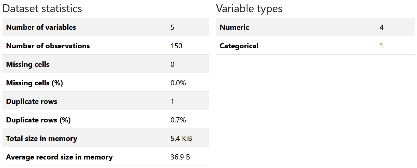
Figure 1.1: Statistics of the data frame.
The report also generates statistics for each individual variable. Figure 1.2 shows the report for sepal length along with its histogram. The report also generates information about interactions between variables in the form of scatter plots and correlation plots.
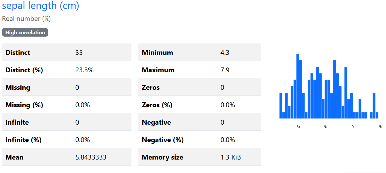
Figure 1.2: Histogram of one of the variables.
While these types of tools can save you a lot of time you may still need to perform some more detailed EDA depending on your needs.