Mistake 9: Not accounting for variance
Before deploying a model into production, you want to be sure you are using the best model for your given use case. In order to find this best model, you may want to compare between different alternatives. To demonstrate this idea, I will use the DIGITS dataset which consists of \(8x8\) images flattened into a feature vector of length \(64\). Each feature consists of an integer between \(0-16\) representing the pixel intensity. Figure 9.1 shows the first digit with class ‘0’.
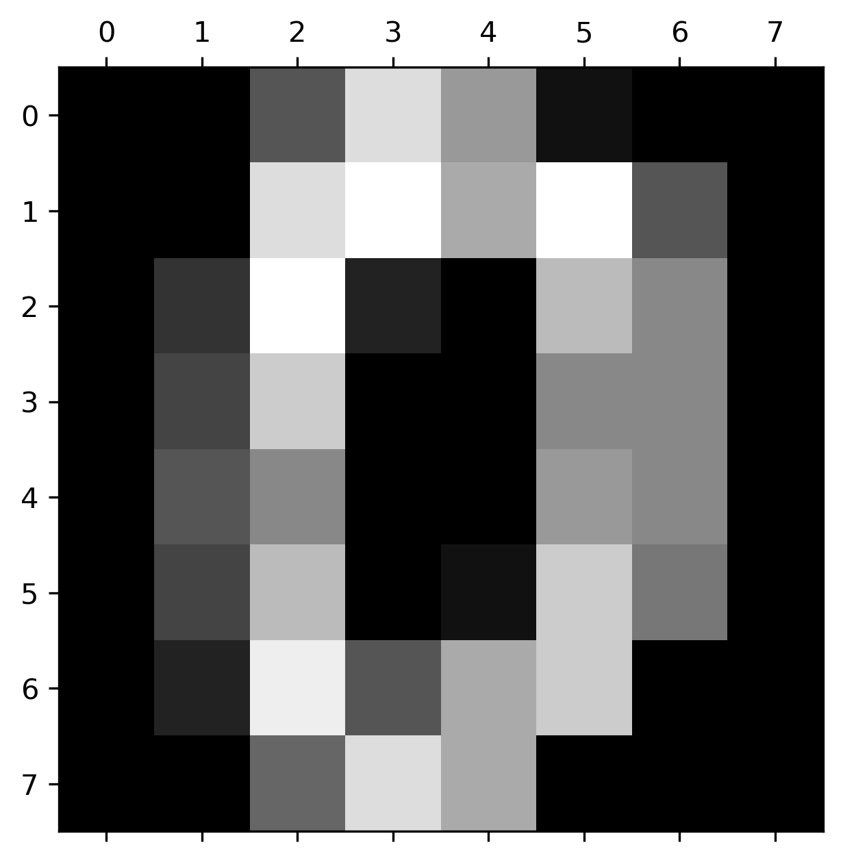
Figure 9.1: Digit 0.
Let’s compare a DecisionTreeClassifier versus a GaussianNB to decide which one is better for digits classification. For the sake of simplicity, I will only use accuracy as the performance metric.
import numpy as np
from sklearn.datasets import load_digits
data = load_digits()

from sklearn.model_selection import train_test_split
X_train, X_test, y_train, y_test = train_test_split(data.data,
                                                    data.target,
                                                    test_size = 0.5,
                                                    random_state = 123)
from sklearn.tree import DecisionTreeClassifier
from sklearn.naive_bayes import GaussianNB
from sklearn.metrics import accuracy_score

tree = DecisionTreeClassifier(random_state=1234)
bayes = GaussianNB()

tree.fit(X_train, y_train)
bayes.fit(X_train, y_train)

predictions_tree = tree.predict(X_test)
predictions_bayes = bayes.predict(X_test)

print(f"Decision Tree accuracy: {accuracy_score(y_test, predictions_tree):.3f}")
print(f"GaussianNB accuracy: {accuracy_score(y_test, predictions_bayes):.3f}")According to those results you may conclude that DecisionTreeClassifier is the best choice. However, it may be the case that if the initial conditions change a little bit (e.g., a slightly different training set), you could get completely different results. And in fact, if you change random_state=1234 to random_state=123 in train_test_split() this time GaussianNB performs better. This is called variance. That is, the results vary from run to run. Then, how can you decide which model is better in the long run? One way is to repeat the experiment several times and select the model that performs better on average. Every time you run the experiment, you randomly partition the train and test sets. In this way, every experiment will have a slightly different train and test sets. This procedure is called Monte Carlo cross-validation. The following code runs \(500\) iterations and computes the average accuracy.
n = 500
accuracy_tree = []
accuracy_bayes = []

for i in range(n):
    X_train, X_test, y_train, y_test = train_test_split(data.data,
                                                    data.target,
                                                    test_size = 0.5,
                                                    random_state = 123 + i)
    tree = DecisionTreeClassifier(random_state=123)
    bayes = GaussianNB()

    tree.fit(X_train, y_train)
    bayes.fit(X_train, y_train)
    predictions_tree = tree.predict(X_test)
    predictions_bayes = bayes.predict(X_test)
    accuracy_tree.append(accuracy_score(y_test, predictions_tree))
    accuracy_bayes.append(accuracy_score(y_test, predictions_bayes))

print(f"Decision Tree accuracy: {np.mean(accuracy_tree):.3f}")
print(f"GaussianNB accuracy: {np.mean(accuracy_bayes):.3f}")Here, we can see that GaussianNB is better on average, contrary to what we thought by only running the experiment one iteration.
train_test_split() in each iteration (random_state = 123 + i). Otherwise the train and test sets will be the same.
Figure 9.2 shows a histogram of the accuracies. Here, we can see that there is some overlap between the two models but on average, GaussianNB is better.
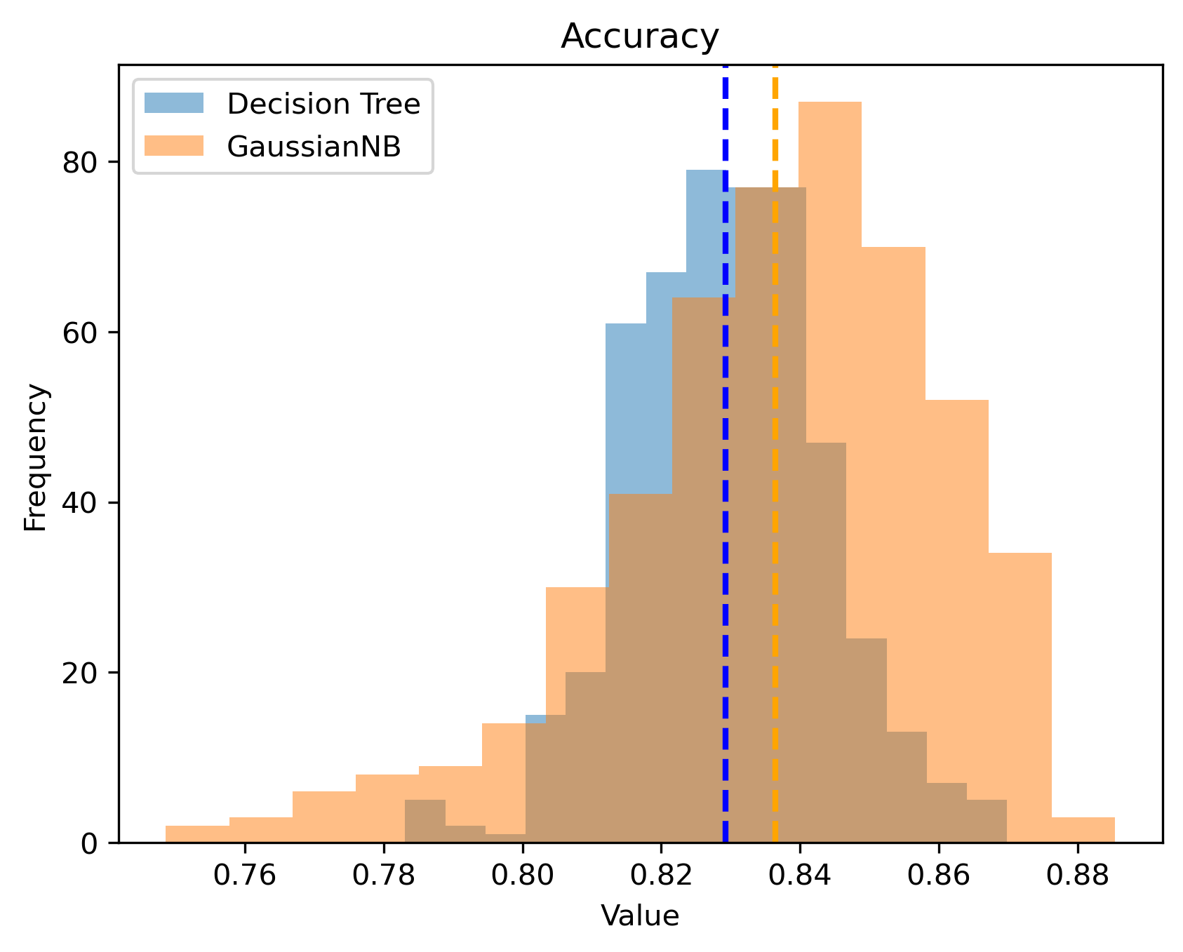
Figure 9.2: Histogram of accuracy.
The difference between the models’ accuracies can be further validated with a Wilcoxon test.
from scipy.stats import wilcoxon
stat, p = wilcoxon(accuracy_tree, accuracy_bayes)
print(f"p-value: {p:.10f}")Since the p-value is \(<0.05\) we can say that the difference between the models is significant. In this example we used Monte Carlo cross-validation to robustly compare two models. However, you should also account for variance when tuning a model’s hyper-parameters, choosing pre-processing methods, data transformations, etc.