Mistake 5: Ignoring differences in scales
As previously mentioned (see Mistake ??), it is always a good idea to perform an exploratory analysis of your data. At this point, you may realize that the features have different scales. For example, let’s load the DIAGNOSTIC dataset and compute some summary statistics with the describe() function. Figure 5.1 shows a summary of the data frame.
from sklearn.datasets import load_breast_cancer
data = load_breast_cancer(as_frame=True)
data.frame.describe()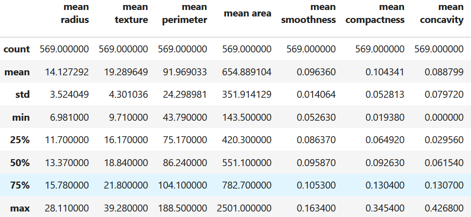
Figure 5.1: Summary statistics of the DIAGNOSTIC dataset.
Here, we can see that the max value of mean concavity is \(0.42\) and the max value of mean area is \(2501\). The later is much larger (in the range of thousands). These differences can have a huge impact in many machine learning models. Specially on those based in distances such as KNN. Suppose we want to compute the distance between two feature vectors \(v_1=[0.21, 2034]\) and \(v_2=[0.19, 1327]\) using the Euclidean distance:
\[\begin{equation} d = \sqrt{(0.21 - 0.19)^2 + (2034 - 1327)^2} \tag{5.1} \end{equation}\]
It is easy to see that the second feature is dominant, making the first one almost irrelevant. One way to deal with this is by normalizing the features so they fall into the same interval, for example \([0-1]\). The following formula can be used to normalize a variable \(X\):
\[\begin{equation} z_i = \frac{X_i - min(X)}{max(X)-min(X)} \tag{5.2} \end{equation}\]
where \(z_i\) is the normalized \(i^{th}\) value and \(max(X)\) and \(min(X)\) are the maximum and minimum values of \(X\). Scikit-learn has the MinMaxScaler() function that does that transformation. The following code split the data into train and test sets. Then, it fits the scaler using the train data and transforms it (line \(10\)). Finally, the test set is transformed as well. Figure 5.2 the summary statistics of the train set after the transformation.
from sklearn.model_selection import train_test_split
from sklearn.preprocessing import MinMaxScaler

X = data.data
y = data.target
X_train, X_test, y_train, y_test = train_test_split(X, y,
                                                    test_size = 0.5,
                                                    random_state = 123)
scaler = MinMaxScaler()
X_train_scaled = scaler.fit_transform(X_train)
X_test_scaled = scaler.transform(X_test)
X_train_scaled_df = pd.DataFrame(X_train_scaled, columns=X.columns)
X_train_scaled_df.describe()
Figure 5.2: Summary statistics of the DIAGNOSTIC dataset after normalization.
Now, the minimum and maximum values of all features are \(0\) and \(1\), respectively. Note that the scaler was fitted using only the train data. That is, the parameters (max, min) were learned from the train set and then applied to the test set. This separation is done to avoid leaking training parameters into the test set (see Mistake 10).
It is worth mentioning that not all models are affected by scale differences. For example, decision trees are immune to differences in scales across features.
MinMaxScaler, StandardScaler, MaxAbsScaler, etc.