Mistake 15: Forgetting that data changes over time
Deploying a model is not the final step in a machine learning pipeline. Data is changing all the time and as a consequence, the model you trained today may not perform the same tomorrow (or even in the same day). Take for example a classifier that predicts if e-mail messages are spam or not. Everyday, spammers develop new tactics to circumvent spam detection systems by modifying the messages’ contents and meta-data. Thus, in order to keep the classifiers up to date, they need to be retrained frequently so they are able to learn the new patterns of spam messages. These types of changes are present in almost any system. The weather conditions change due to global warming, companies’ sales change when introducing new products, sensors’ data deviate due to vibrations, and so on. Thus, after deploying a model, some mechanisms should be implemented to monitor its behavior and if data deviations are detected, apply corrections. In machine learning, data drift refers to the change in statistical properties over time of the features and/or response variables (labels, or values for regression).
There are three main types of data drift.
Covariate drift. This happens when the distribution (for example, the average) of features changes over time.
Prior probability drift. This can happen when the distribution of the response variable changes. For example, an increase in the proportion of spam messages compared to the previous year.
Concept drift. When the relationship between features and the response variable changes over time.
Detecting those changes include strategies like monitoring variable distributions, statistical tests, using auto-encoders, and so on. Once a change is detected, the model can be retrained or adapted. The topic of data drift is very extensive and encompasses a broad range of techniques for monitoring and adaptation. The interested reader is referred to these reviews on the topic (Lu et al. 2018) and (Gama et al. 2014).
One of the most common techniques to detect data drift in numeric features is the Wasserstein distance. Intuitively, it measures the required effort to transform one distribution into another.
\[\begin{equation} W(P, Q) = \int_{-\infty}^{\infty} \left| F_P(x) - F_Q(x) \right| \, dx \tag{15.1} \end{equation}\]
where \(F_P(x)\) and \(F_Q(x)\) are the cumulative distribution functions.
The following code generates an array (reference_data) of size \(1000\) with random values drawn from a normal distribution with mean \(0\) and a standard deviation of \(1\). To simulate data drift, a second array (new_data) is randomly generated, but this time the mean is \(1.5\) instead of \(0\).
import numpy as np
from scipy.stats import wasserstein_distance

# Set random seed for reproducibility
np.random.seed(123)

# Generate example data.
reference_data = np.random.normal(loc=0, scale=1, size=1000)
new_data = np.random.normal(loc=1.5, scale=1, size=1000)
Figure 15.1 shows the distribution of the two arrays. While the reference data is centered at \(0\), the mean of the new data ‘moved’ to the right approximately \(1.5\) units.
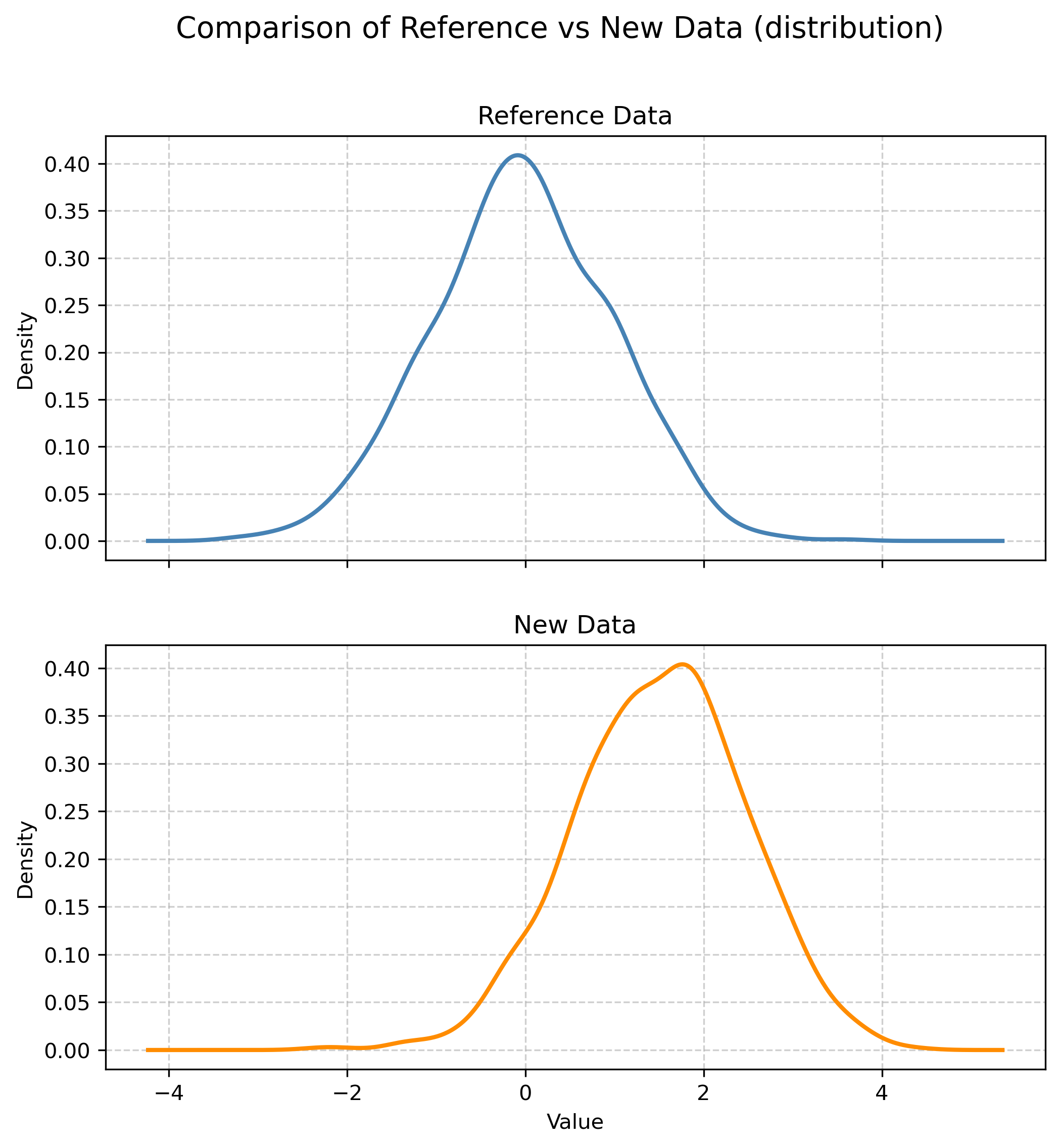
Figure 15.1: Comparison of the distribution between the reference and new data.
The following code uses the wasserstein_distance() function from the scipy library to compute the Wasserstein distance between the two arrays.
# Calculate Wasserstein Distance.
distance = wasserstein_distance(reference_data, new_data)
print(f"Wasserstein Distance: {distance:.4f}")Here, you can see that the distance is \(1.5480\). The closest to zero, the smaller the data drift. In this example the data drift was considerable. Based on this distance, you can decide if your model needs to be retrained. The threshold to decide if retraining is required will depend on your specific application. You can try changing the loc and scale parameters in new_data = np.random.normal(loc=1.5, scale=1, size=1000) and see how the Wasserstein distance changes accordingly.