Chapter 5 Preprocessing Behavioral Data
preprocessing.R
Behavioral data comes in many flavors and forms, but when training predictive models, the data needs to be in a particular format. Some sources of variation when collecting data are:
Sensors’ format. Each type of sensor and manufacturer stores data in a different format. For example, .csv files, binary files, images, proprietary formats, etc.
Sampling rate. The sampling rate is how many measurements are taken per unit of time. For example, a heart rate sensor may return a single value every second, thus, the sampling rate is \(1\) Hz. An accelerometer that captures \(50\) values per second has a sampling rate of \(50\) Hz.
Scales and ranges. Some sensors may return values in degrees (e.g., a temperature sensor) while others may return values in some other scale, for example, in centimeters for a proximity sensor. Furthermore, ranges can also vary. That is, a sensor may capture values in the range of \(0-1000\), for example.
During the data exploration step (chapter 4) we may also find that values are missing, inconsistent, noisy, and so on, thus, we also need to take care of that.
This chapter provides an overview of some common methods used to clean and preprocess the data before one can start training reliable models.
5.1 Missing Values
Many datasets will have missing values and we need ways to identify and deal with that. Missing data could be due to faulty sensors, processing errors, unavailable information, and so on. In this section, I present some tools that ease the identification of missing values. Later, some imputation methods used to fill in the missing values are presented.
To demonstrate some of these concepts, the SHEEP GOATS dataset (Kamminga et al. 2017) will be used. Due to its big size, the files of this dataset are not included with the accompanying book files but they can be downloaded from https://easy.dans.knaw.nl/ui/datasets/id/easy-dataset:76131. The data were released as part of a study about animal behaviors. The researchers placed inertial sensors on sheep and goats and tracked their behavior during one day. They also video-recorded the session and annotated the data with different types of behaviors such as grazing, fighting, scratch-biting, etc. The device was placed on the neck with a random orientation and it collected acceleration, orientation, magnetic field, temperature, and barometric pressure. Figure 5.1 shows a schematic view of the setting.

FIGURE 5.1: Device placed on the neck of the sheep. (Author: LadyofHats. Source: Wikipedia (CC0 1.0)).
We will start by loading a .csv file that corresponds to one of the sheep and check if there are missing values. The naniar package (Tierney et al. 2019) offers a set of different functions to explore and deal with missing values. The gg_miss_var() function allows you to quickly check which variables have missing values and how many. The following code loads the data and then plots the number of missing values in each variable.
library(naniar)

# Path to S1.csv file.
datapath <- file.path(datasets_path,
                      "sheep_goats","S1.csv")

# Can take some seconds to load since the file is big.
df <- read.csv(datapath, stringsAsFactors = TRUE)

# Plot missing values.
gg_miss_var(df)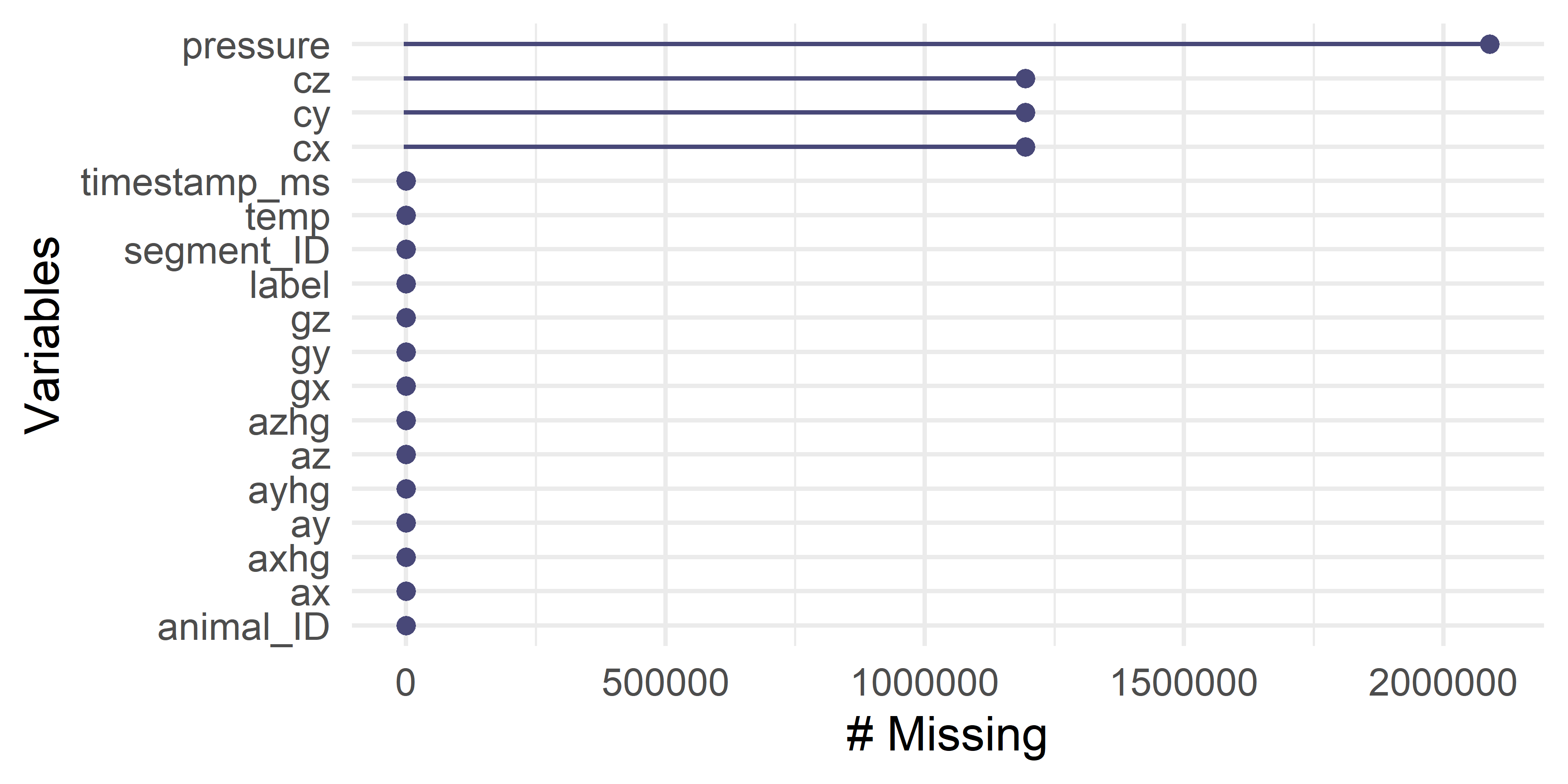
FIGURE 5.2: Missing values counts.
Figure 5.2 shows the resulting output. The plot shows that there are missing values in four variables: pressure, cz, cy, and cx. The last three correspond to the compass (magnetometer). For pressure, the number of missing values is more than \(2\) million! For the rest, it is a bit less (more than \(1\) million).
To further explore this issue, we can plot each observation in a row with the function vis_miss().
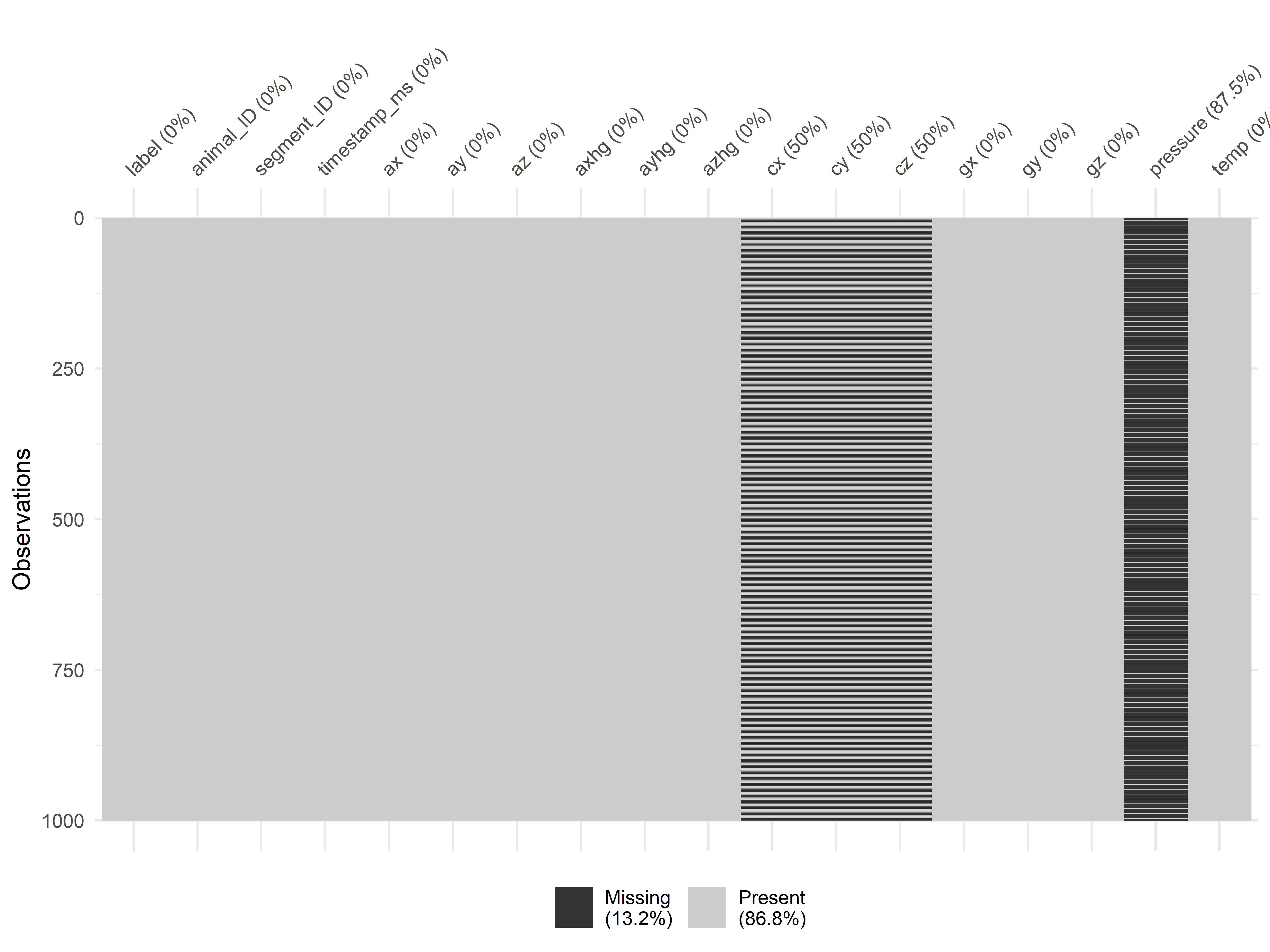
FIGURE 5.3: Rows with missing values.
Figure 5.3 shows every observation per row and missing values are black colored (if any). From this image, it seems that missing values are systematic. It looks like there is a clear stripes pattern, especially for the compass variables. Based on these observations, it doesn’t look like random sensor failures or random noise.
If we explore the data frame’s values, for example with the RStudio viewer (Figure 5.4), two things can be noted. First, for the compass values, there is a missing value for each present value. Thus, it looks like \(50\%\) of compass values are missing. For pressure, it seems that there are \(7\) missing values for each available value.
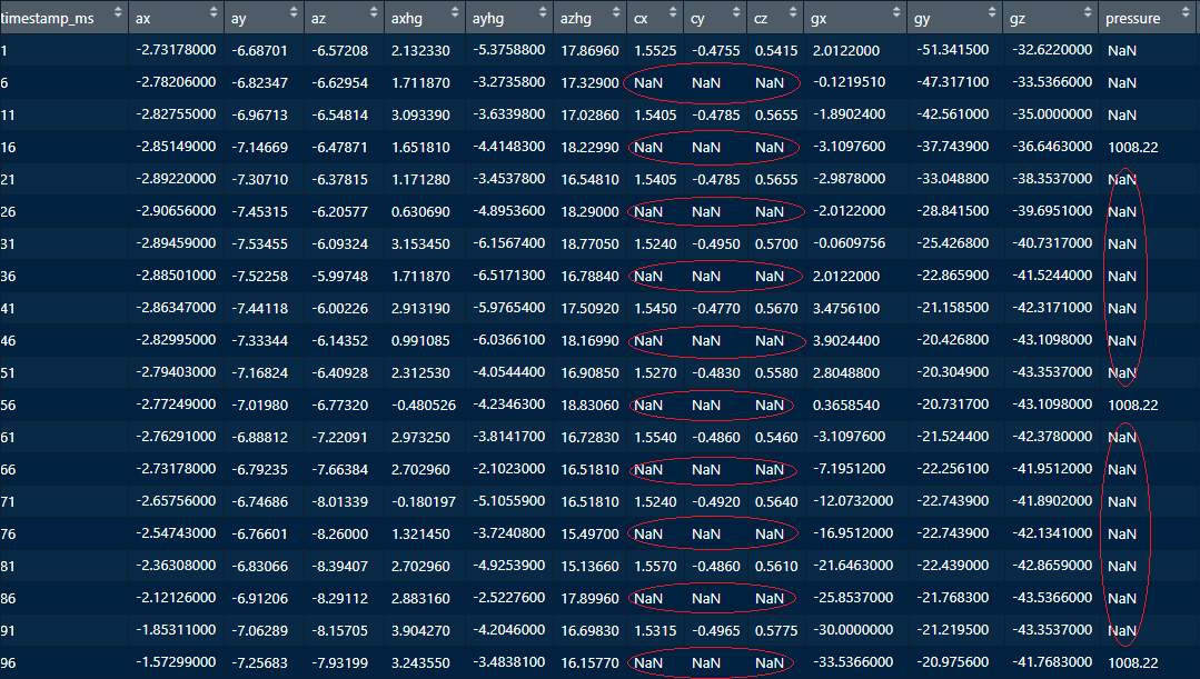
FIGURE 5.4: Displaying the data frame in RStudio. Source: Data from Kamminga, MSc J.W. (University of Twente) (2017): Generic online animal activity recognition on collar tags. DANS. https://doi.org/10.17026/dans-zp6-fmna
So, what could be the root cause of those missing values? Remember that at the beginning of this chapter it was mentioned that one of the sources of variation is sampling rate. If we look at the data set documentation, all sensors have a sampling rate of \(200\) Hz except for the compass and the pressure sensor. The compass has a sampling rate of \(100\) Hz. That is half compared to the other sensors! This explains why \(50\%\) of the rows are missing. Similarly, the pressure sensor has a sampling rate of \(25\) Hz. By visualizing and then inspecting the missing data, we have just found out that the missing values are not caused by random noise or sensor failures but because some sensors are not as fast as others!
Now that we know there are missing values we need to decide what to do with them. The following subsection lists some ways to deal with missing values.
5.1.1 Imputation
Imputation is the process of filling in missing values. One of the reasons for imputing missing values is that some predictive models cannot deal with missing data. Another reason is that it may help in increasing the predictions’ performance, for example, if we are trying to predict the sheep behavior from a discrete set of categories based on the inertial data. There are different ways to handle missing values:
Discard rows. If the rows with missing values are not too many, they can simply be discarded.
Mean value. Fill the missing values with the mean value of the corresponding variable. This method is simple and can be effective. One of the problems with this method is that it is sensitive to outliers (as it is the arithmetic mean).
Median value. The median is robust against outliers, thus, it can be used instead of the arithmetic mean to fill the gaps.
Replace with the closest value. For timeseries data, as is the case of the sheep readings, one could also replace missing values with the closest known value.
Predict the missing values. Use the other variables to predict the missing one. This can be done by training a predictive model. A regressor if the variable is numeric or a classifier if the variable is categorical.
Another problem with the mean and median values is that they can be correlated with other variables, for example, with the class that we want to predict. One way to avoid this, is to compute the mean (or median) for each class, but still, some hidden correlations may bias the estimates.
In R, the simputation package (van der Loo 2019) has implemented various imputation techniques including: group-wise median imputation, model-based with linear regression, random forests, etc. The following code snippet (complete code is in preprocessing.R) uses the impute_lm() method to impute the missing values in the sheep data using linear regression.
library(simputation)

# Replace NaN with NAs.
# Since missing values are represented as NaN,
# first we need to replace them with NAs.

# Code to replace NaN with NA was taken from Hong Ooi:
# https://stackoverflow.com/questions/18142117/#
# how-to-replace-nan-value-with-zero-in-a-huge-data-frame/18143097
is.nan.data.frame <- function(x)do.call(cbind, lapply(x, is.nan))
df[is.nan(df)] <- NA

# Use simputation package to impute values.
# The first 4 columns are removed since we
# do not want to use them as predictor variables.
imp_df <- impute_lm(df[,-c(1:4)],
                    cx + cy + cz + pressure ~ . - cx - cy - cz - pressure)
# Print summary.
summary(imp_df)
Originally, the missing values are encoded as NaN but in order to use the simputation package functions, we need them as NA. First, NaNs are replaced with NA. The first argument of impute_lm() is a data frame and the second argument is a formula. We discard the first \(4\) variables of the data frame since we do not want to use them as predictors. The left-hand side of the formula (everything before the ~ symbol) specifies the variables we want to impute. The right-hand side specifies the variables used to build the linear models. The ‘.’ indicates that we want to use all variables while the ‘-’ is used to specify variables that we do not want to include. The vignettes10 of the package contain more detailed examples.
5.2 Smoothing
Smoothing comprises a set of algorithms with the aim of highlighting patterns in the data or as a preprocessing step to clean the data and remove noise. These methods are widely used on timeseries data but also with spatio-temporal data such as images. With timeseries data, they are often used to emphasize long-term patterns and reduce short-term signal artifacts. For example, in Figure 5.511 a stock chart was smoothed using two methods: moving average and exponential moving average. The smoothed versions make it easier to spot the overall trend rather than focusing on short-term variations.
![Stock chart with two smoothed versions. One with moving average and the other one with an exponential moving average. (Author: Alex Kofman. Source: Wikipedia (CC BY-SA 3.0) [https://creativecommons.org/licenses/by-sa/3.0/legalcode]).](images/smoothing_stock.png)
FIGURE 5.5: Stock chart with two smoothed versions. One with moving average and the other one with an exponential moving average. (Author: Alex Kofman. Source: Wikipedia (CC BY-SA 3.0) [https://creativecommons.org/licenses/by-sa/3.0/legalcode]).
The most common smoothing method for timeseries is the simple moving average. With this method, the first element of the resulting smoothed series is computed by taking the average of the elements within a window of predefined size. The window’s position starts at the first element of the original series. The second element is computed in the same way but after moving the window one position to the right. Figure 5.6 shows this procedure on a series with \(5\) elements and a window size of size \(3\). After the third iteration, it is not possible to move the window one more step to the right while covering \(3\) elements since the end of the timeseries has been reached. Because of this, the smoothed series will have some missing values at the end. Specifically, it will have \(w-1\) fewer elements where \(w\) is the window size. A simple solution is to compute the average of the elements covered by the window even if they are less than the window size.
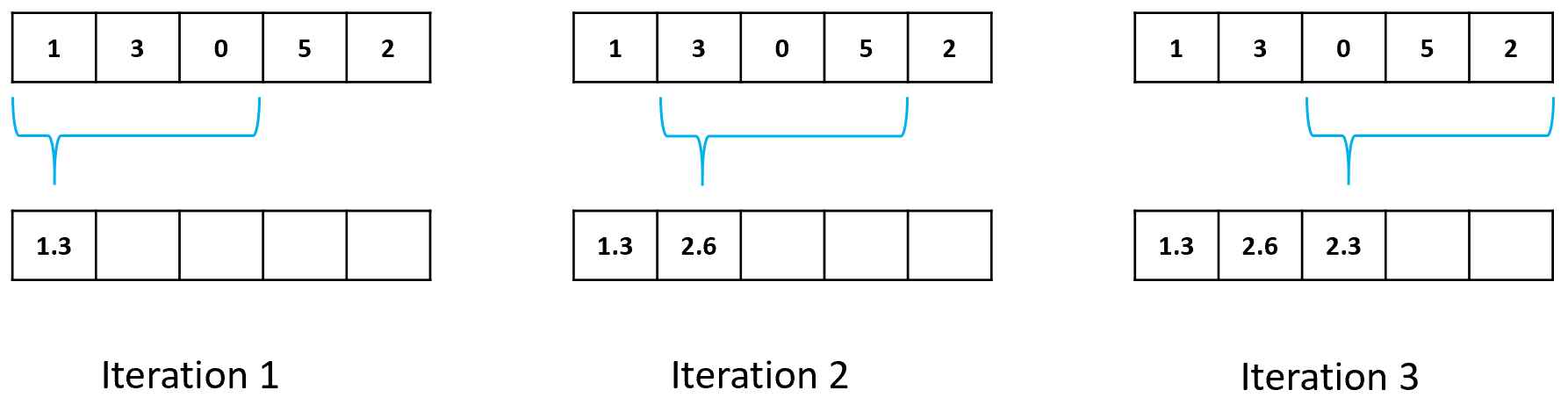
FIGURE 5.6: Simple moving average step by step with window size = 3. Top: original array; bottom: smoothed array.
In the previous example the average is taken from the elements to the right of the pointer. There is a variation called centered moving average in which the center point of the window has the same elements to the left and right (Figure 5.7). Note that with this version of moving average some values at the beginning and at the end will be empty. Also note that the window size should be odd. In practice, both versions produce very similar results.
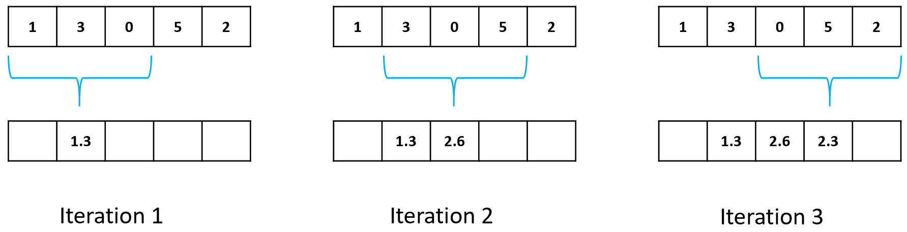
FIGURE 5.7: Centered moving average step by step with window size = 3.
In the preprocessing.R script, the function movingAvg() implements the simple moving average procedure. In the following code, note that the output vector will have the same size as the original one, but the last elements will contain NA values when the window cannot be moved any longer to the right.
movingAvg <- function(x, w = 5){
  # Applies moving average to x with a window of size w.
  n <- length(x) # Total number of points.
  smoothedX <- rep(NA, n)

  for(i in 1:(n-w+1)){
    smoothedX[i] <- mean(x[i:(i-1+w)])
  }

  return(smoothedX)
}
We can apply this function to a segment of accelerometer data from the SHEEP AND GOATS data set.
datapath <- "../Sheep/S1.csv"
df <- read.csv(datapath)

# Only select a subset of the whole series.
dfsegment <- df[df$timestamp_ms < 6000,]
x <- dfsegment$ax

# Compute simple moving average with a window of size 21.
smoothed <- movingAvg(x, w = 21)
Figure 5.8 shows the result after plotting both the original vector and the smoothed one. It can be observed that many of the small peaks are no longer present in the smoothed version. The window size is a parameter that needs to be defined by the user. If it is set too large some important information may be lost from the signal.
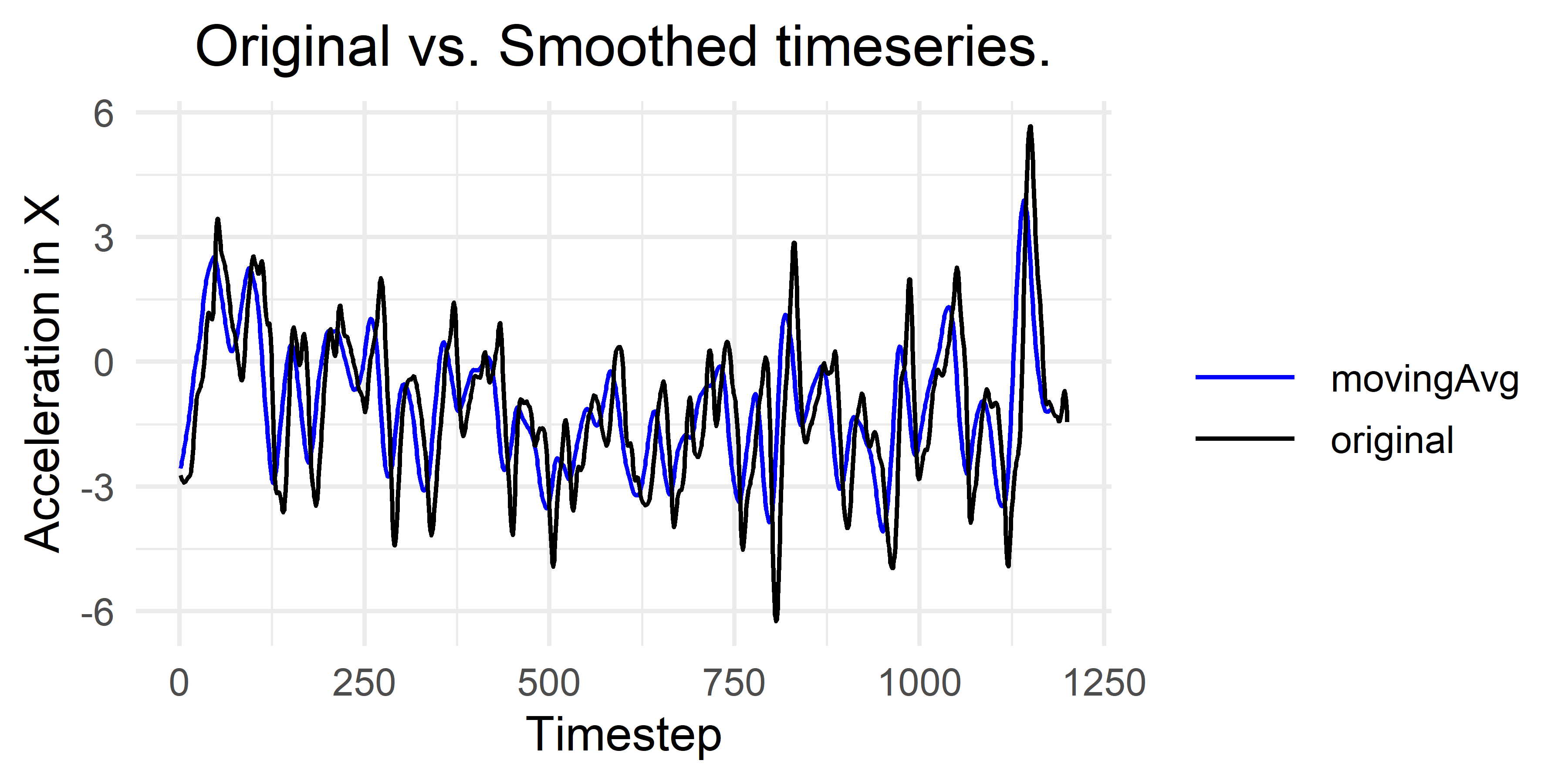
FIGURE 5.8: Original time series and smoothed version using a moving average window of size 21.
One of the disadvantages of this method is that the arithmetic mean is sensitive to noise. Instead of computing the mean, one can use the median which is more robust against outlier values. There also exist other derived methods (not covered here) such as weighted moving average and exponential moving average12 which assign more importance to data points closer to the central point in the window. Smoothing a signal before feature extraction is a common practice and is used to remove some of the unwanted noise.
5.3 Normalization
Having variables on different scales can have an impact during learning and at inference time. Consider a study where the data was collected using a wristband that has a light sensor and an accelerometer. The measurement unit of the light sensor is lux whereas the accelerometer’s is \(m/s^2\). After inspecting the dataset, you realize that the min and max values of the light sensor are \(0\) and \(155\), respectively. The min and max values for the accelerometer are \(-0.4\) and \(7.45\), respectively. Why is this a problem? Well, several learning methods are based on distances such as \(k\)-NN and Nearest centroid thus, distances will be more heavily affected by bigger scales. Furthermore, other methods like neural networks (covered in chapter 8) are also affected by different scales. They have a harder time learning their parameters (weights) when data is not normalized. On the other hand, some methods are not affected, for example, tree-based learners such as decision trees and random forests. Since most of the time you may want to try different methods, it is a good idea to normalize your predictor variables.
A common normalization technique is to scale all the variables between \(0\) and \(1\). Suppose there is a numeric vector \(x\) that you want to normalize between \(0\) and \(1\). Let \(max(x)\) and \(min(x)\) be the maximum and minimum values of \(x\). The following can be used to normalize the \(i^{th}\) value of \(x\):
\[\begin{equation} z_i = \frac{x_i - min(x)}{max(x)-min(x)} \end{equation}\]
where \(z_i\) is the new normalized \(i^{th}\) value. Thus, the formula is applied to every value in \(x\). The \(max(x)\) and \(min(x)\) values are parameters learned from the data. Notice that if you will split your data into training and test sets the max and min values (the parameters) are learned only from the train set and then used to normalize both the train and test set. This is to avoid information injection (section 5.5). Be also aware that after the parameters are learned from the train set, and once the model is deployed in production, it is likely that some input values will be ‘out of range’. If the train set is not very representative of what you will find in real life, some values will probably be smaller than the learned \(min(x)\) and some will be greater than the learned \(max(x)\). Even if the train set is representative of the real-life phenomenon, there is nothing that will prevent some values to be out of range. A simple way to handle this is to truncate the values. In some cases, we do know what are the possible minimum and maximum values. For example in image processing, images are usually represented as color intensities between \(0\) and \(255\). Here, we know that the min value cannot be less than \(0\) and the max value cannot be greater than \(255\).
Let’s see an example using the HOME TASKS dataset. The following code first loads the dataset and prints a summary of the first \(4\) variables.
# Load home activities dataset.
dataset <- read.csv(file.path(datasets_path,
                              "home_tasks",
                              "sound_acc.csv"),
                    stringsAsFactors = T)

# Check first 4 variables' min and max values.
summary(dataset[,1:4])

#>                label        v1_mfcc1      v1_mfcc2         v1_mfcc3
#> brush_teeth     :180   Min.   :103   Min.   :-17.20   Min.   :-20.90
#> eat_chips       :282   1st Qu.:115   1st Qu.: -8.14   1st Qu.: -7.95
#> mop_floor       :181   Median :120   Median : -3.97   Median : -4.83
#> sweep           :178   Mean   :121   Mean   : -4.50   Mean   : -5.79
#> type_on_keyboard:179   3rd Qu.:126   3rd Qu.: -1.30   3rd Qu.: -3.09
#> wash_hands      :180   Max.   :141   Max.   :  8.98   Max.   :  3.27
#> watch_tv        :206
Since label is a categorical variable, the class counts are printed. For the three remaining variables, we get some statistics including their min and max values. As we can see, the min value of v1_mfcc1 is very different from the min value of v1_mfcc2 and the same is true for the maximum values. Thus, we want all variables to be between \(0\) and \(1\) in order to use classification methods sensitive to different scales. Let’s assume we want to train a classifier with this data so we divide it into train and test sets:
# Divide into 50/50% train and test set.
set.seed(1234)
folds <- sample(2, nrow(dataset), replace = T)
trainset <- dataset[folds == 1,]
testset <- dataset[folds == 2,]
Now we can define a function that normalizes every numeric or integer variable. If the variable is not numeric or integer it will skip them. The function will take as input a train set and a test set. The parameters (max and min) are learned from the train set and used to normalize both, the train and test sets.
# Define a function to normalize the train and test set
# based on the parameters learned from the train set.
normalize <- function(trainset, testset){

  # Iterate columns
  for(i in 1:ncol(trainset)){

    c <- trainset[,i] # trainset column
    c2 <- testset[,i] # testset column

    # Skip if the variable is not numeric or integer.
    if(class(c) != "numeric" && class(c) != "integer")next;

    # Learn the max value from the trainset's column.
    max <- max(c, na.rm = T)
    # Learn the min value from the trainset's column.
    min <- min(c, na.rm = T)

    # If all values are the same set it to max.
    if(max==min){
      trainset[,i] <- max
      testset[,i] <- max
    }
    else{

      # Normalize trainset's column.
      trainset[,i] <- (c - min) / (max - min)

      # Truncate max values in testset.
      idxs <- which(c2 > max)
      if(length(idxs) > 0){
        c2[idxs] <- max
      }

      # Truncate min values in testset.
      idxs <- which(c2 < min)
      if(length(idxs) > 0){
        c2[idxs] <- min
      }

      # Normalize testset's column.
      testset[,i] <- (c2 - min) / (max - min)
    }
  }

  return(list(train=trainset, test=testset))
}
Now we can use the previous function to normalize the train and test sets. The function returns a list of two elements: a normalized train and test sets.
# Call our function to normalize each set.
normalizedData <- normalize(trainset, testset)

# Inspect the normalized train set.
summary(normalizedData$train[,1:4])

#>                label        v1_mfcc1        v1_mfcc2        v1_mfcc3
#> brush_teeth     : 88   Min.   :0.000   Min.   :0.000   Min.   :0.000
#> eat_chips       :139   1st Qu.:0.350   1st Qu.:0.403   1st Qu.:0.527
#> mop_floor       : 91   Median :0.464   Median :0.590   Median :0.661
#> sweep           : 84   Mean   :0.474   Mean   :0.568   Mean   :0.616
#> type_on_keyboard: 94   3rd Qu.:0.613   3rd Qu.:0.721   3rd Qu.:0.730
#> wash_hands      :102   Max.   :1.000   Max.   :1.000   Max.   :1.000
#> watch_tv        : 99

# Inspect the normalized test set.
summary(normalizedData$test[,1:4])
#>                label        v1_mfcc1         v1_mfcc2        v1_mfcc3
#> brush_teeth     : 92   Min.   :0.0046   Min.   :0.000   Min.   :0.000
#> eat_chips       :143   1st Qu.:0.3160   1st Qu.:0.421   1st Qu.:0.500
#> mop_floor       : 90   Median :0.4421   Median :0.606   Median :0.644
#> sweep           : 94   Mean   :0.4569   Mean   :0.582   Mean   :0.603
#> type_on_keyboard: 85   3rd Qu.:0.5967   3rd Qu.:0.728   3rd Qu.:0.724
#> wash_hands      : 78   Max.   :0.9801   Max.   :1.000   Max.   :1.000
#> watch_tv        :107
Now, the variables on the train set are exactly between \(0\) and \(1\) for all numeric variables. For the test set, not all min values will be exactly \(0\) but a bit higher. Conversely, some max values will be lower than \(1\). This is because the test set may have a min value that is greater than the min value of the train set and a max value that is smaller than the max value of the train set. However, after normalization, all values are guaranteed to be within \(0\) and \(1\).
5.4 Imbalanced Classes
Ideally, classes will be uniformly distributed, that is, there is approximately the same number of instances per class. In real-life (as always), this is not the case. And in many situations (more often than you may think), class counts are heavily skewed. When this happens the dataset is said to be imbalanced. Take as an example, bank transactions. Most of them will be normal, whereas a small percent will be fraudulent. In the medical field this is very common. It is easier to collect samples from healthy individuals compared to samples from individuals with some rare conditions. For example, a database may have thousands of images from healthy tissue but just a dozen with signs of cancer. Of course, having just a few cases with diseases is a good thing for the world! but not for machine learning methods. This is because predictive models will try to learn their parameters such that the error is reduced, and most of the time this error is based on accuracy. Thus, the models will be biased towards making correct predictions for the majority classes (the ones with higher counts) while paying little attention to minority classes. This is a problem because for some applications we are more interested in detecting the minority classes (illegal transactions, cancer cases, etc.).
Suppose a given database has \(998\) instances with class ‘no cancer’ and only \(2\) instances with class ‘cancer’. A trivial classifier that always predicts ‘no cancer’ will have an accuracy of \(98.8\%\) but will not be able to detect any of the ‘cancer’ cases! So, what can we do?
Collect more data from the minority class. In practice, this can be difficult, expensive, etc. or just impossible because the study was conducted a long time ago and it is no longer possible to replicate the context.
Delete data from the majority class. Randomly discard instances from the majority class. In the previous example, we could discard \(996\) instances of type ‘no cancer’. The problem with this is that we end up with insufficient data to learn good predictive models. If you have a huge dataset this can be an option, but in practice, this is rarely the case and you have the risk of having underrepresented samples.
Create synthetic data. One of the most common solutions is to create synthetic data from the minority classes. In the following sections two methods that do that will be discussed: random oversampling and Synthetic Minority Oversampling Technique (SMOTE).
Adapt your learning algorithm. Another option is to use an algorithm that takes into account class counts and weights them accordingly. This is called cost-sensitive classification. For example, the
rpart()method to train decision trees has aweightparameter which can be used to assign more weight to minority classes. When training neural networks it is also possible to assign different weights to different classes.
The following two subsections cover two techniques to create synthetic data.
5.4.1 Random Oversampling
shiny_random-oversampling.Rmd
This method consists of duplicating data points from the minority class. The following code will create an imbalanced dataset with \(200\) instances of class ‘class1’ and only \(15\) instances of class ‘class2’.
set.seed(1234)

# Create random data
n1 <- 200 # Number of points of majority class.
n2 <- 15 # Number of points of minority class.

# Generate random values for class1.
x <- rnorm(mean = 0, sd = 0.5, n = n1)
y <- rnorm(mean = 0, sd = 1, n = n1)
df1 <- data.frame(label=rep("class1", n1),
                  x=x, y=y, stringsAsFactors = T)

# Generate random values for class2.
x2 <- rnorm(mean = 1.5, sd = 0.5, n = n2)
y2 <- rnorm(mean = 1.5, sd = 1, n = n2)
df2 <- data.frame(label=rep("class2", n2),
                  x=x2, y=y2, stringsAsFactors = T)

# This is our imbalanced dataset.
imbalancedDf <- rbind(df1, df2)

# Print class counts.
summary(imbalancedDf$label)
#> class1 class2
#<    200     15
If we want to exactly balance the class counts, we will need \(185\) additional instances of type ‘class2’. We can use our well known sample() function to pick \(185\) points from data frame df2 (which contains only instances of class ‘class2’) and store them in new.points. Notice the replace = T parameter. This allows the function to pick repeated elements. Then, the new data points are appended to the imbalanced data set which now becomes balanced.
# Generate new points from the minority class.
new.points <- df2[sample(nrow(df2), size = 185, replace = T),]

# Add new points to the imbalanced dataset and save the
# result in balancedDf.
balancedDf <- rbind(imbalancedDf, new.points)

# Print class counts.
summary(balancedDf$label)
#> class1 class2
#>   200    200
The code associated with this chapter includes a shiny app13 shiny_random-oversampling.Rmd. Shiny apps are interactive web applications. This shiny app graphically demonstrates how random oversampling works. Figure 5.9 depicts the shiny app. The user can move the slider to generate new data points. Please note that the boundaries do not change as the number of instances increases (or decreases). This is because the new points are just duplicates so they overlap with existing ones.
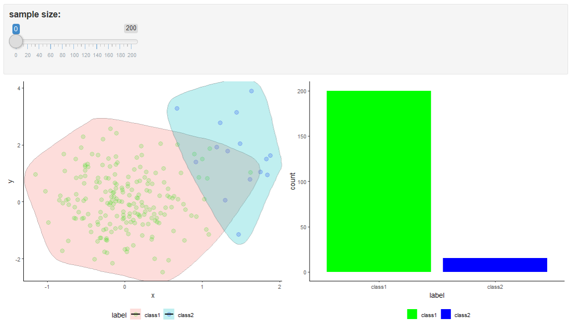
FIGURE 5.9: Shiny app with random oversampling example.
Random oversampling is simple and effective in many cases. A potential problem is that the models can overfit since there are many duplicate data points. To overcome this, the SMOTE method creates entirely new instances instead of duplicating them.
5.4.2 SMOTE
shiny_smote-oversampling.Rmd
SMOTE is another method that can be used to augment the data points from the minority class (Chawla et al. 2002). One of the limitations of random oversampling is that it creates duplicates. This has the effect of having fixed boundaries and the classifiers can overspecialize. To avoid this, SMOTE creates entirely new data points.
SMOTE operates on the feature space (on the predictor variables). To generate a new point, take the difference between a given point \(a\) (taken from the minority class) and one of its randomly selected nearest neighbors \(b\). The difference is multiplied by a random number between \(0\) and \(1\) and added to \(a\). This has the effect of selecting a point along the line between \(a\) and \(b\). Figure 5.10 illustrates the procedure of generating a new point in two dimensions.
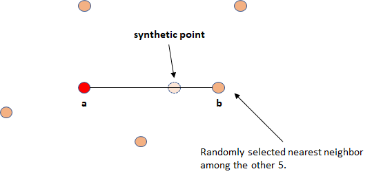
FIGURE 5.10: Synthetic point generation.
The number of nearest neighbors \(k\) is a parameter defined by the user. In their original work (Chawla et al. 2002), the authors set \(k=5\). Depending on how many new samples need to be generated, \(k'\) neighbors are randomly selected from the original \(k\) nearest neighbors. For example, if \(200\%\) oversampling is needed, \(k'=2\) neighbors are selected at random out of the \(k=5\) and one data point is generated with each of them. This is performed for each data point in the minority class.
An implementation of SMOTE is also provided in auxiliary_functions/functions.R. An example of its application can be found in preprocessing.R in the corresponding directory of this chapter’s code. The smote.class(completeDf, targetClass, N, k) function has several arguments. The first one is the data frame that contains the minority and majority class, that is, the complete dataset. The second argument is the minority class label. The third argument N is the percent of smote and the last one (k) is the number of nearest neighbors to consider.
The following code shows how the function smote.class() can be used to generate new points from the imbalanced dataset that was introduced in the previous section ‘Random Oversampling’. Recall that it has \(200\) points of class ‘class1’ and \(15\) points of class ‘class2’.
# To balance the dataset, we need to oversample 1200%.
# This means that the method will create 12 * 15 new points.
ceiling(180 / 15) * 100
#> [1] 1200

# Percent to oversample.
N <- 1200

# Generate new data points.
synthetic.points <- smote.class(imbalancedDf,
                                targetClass = "class2",
                                N = N,
                                k = 5)$synthetic

# Append the new points to the original dataset.
smote.balancedDf <- rbind(imbalancedDf,
                          synthetic.points)

# Print class counts.
summary(smote.balancedDf$label)
#> class1 class2
#>    200    195
The parameter N is set to \(1200\). This will create \(12\) new data points for every minority class instance (\(15\)). Thus, the method will return \(180\) instances. In this case, \(k\) is set to \(5\). Finally, the new points are appended to the imbalanced dataset having a total of \(195\) samples of class ‘class2’.
Again, a shiny app is included with this chapter’s code. Figure 5.11 shows the distribution of the original points and after applying SMOTE. Note how the boundary of ‘class2’ changes after applying SMOTE. It slightly spans in all directions. This is particularly visible in the lower right corner. This boundary expansion is what allows the classifiers to generalize better as compared to training them using random oversampled data.
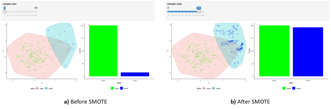
FIGURE 5.11: Shiny app with SMOTE example. a) Before applying SMOTE. b) After applying SMOTE.
5.5 Information Injection
The purpose of dividing the data into train/validation/test sets is to accurately estimate the generalization performance of a predictive model when it is presented with previously unseen data points. So, it is advisable to construct such set splits in a way that they are as independent as possible. Often, before training a model and generating predictions, the data needs to be preprocessed. Preprocessing operations may include imputing missing values, normalizing, and so on. During those operations, some information can be inadvertently transferred from the train to the test set thus, violating the assumption that they are independent.
Suppose that as one of the preprocessing steps, you need to subtract the mean value of a feature for each instance. For now, suppose a dataset has a single feature \(x\) of numeric type and a categorical response variable \(y\). The dataset has \(n\) rows. As a preprocessing step, you decide that you need to subtract the mean of \(x\) from each data point. Since you want to predict \(y\) given \(x\), you train a classifier by splitting your data into train and test sets as usual. So you proceed with the steps depicted in Figure 5.12.
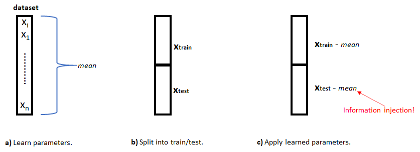
FIGURE 5.12: Information injection example. a) Parameters are learned from the entire dataset. b) The dataset is split intro train/test sets. c) The learned parameters are applied to both sets and information injection occurs.
First, (a) you compute the \(mean\) value of the of variable \(x\) from the entire dataset. This \(mean\) is known as the parameter. In this case, there is only one parameter but there could be several. For example, we could additionally need to compute the standard deviation. Once we know the mean value, the dataset is divided into train and test sets (b). Finally, the \(mean\) is subtracted from each element in both train and test sets (c). Without realizing, we have transferred information from the train set to the test set! But, how did this happen? Well, the mean parameter was computed using information from the entire dataset. Then, that \(mean\) parameter was used on the test set, but it was calculated using data points that also belong to that same test set!
Figure 5.13 shows how to correctly do the preprocessing to avoid information injection. The dataset is first split (a). Then, the \(mean\) parameter is calculated only with data points from the train set. Finally, the mean parameter is subtracted from both sets. Here, the mean contains information only from the train set.
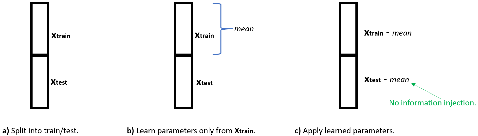
FIGURE 5.13: No information injection example. a) The dataset is first split into train/test sets. b) Parameters are learned only from the train set. c) The learned parameters are applied to the test set.
In the previous example, we assumed that the dataset was split into train and test sets only once. The same idea applies when performing \(k\)-fold cross-validation. In each of the \(k\) iterations, the preprocessing parameters need to be learned only from the train split.
5.6 One-hot Encoding
Several algorithms need some or all of their input variables to be in numeric format, either the response and/or predictor variables. In R, for most classification algorithms, the class is usually encoded as a factor but some implementations may require it to be numeric. Sometimes there may be categorical variables as predictors such as gender (‘male’, ‘female’). Some algorithms need those to be in numeric format because they, for example, are based on distance computations such as \(k\)-NN. Other models need to perform arithmetic operations on the predictor variables like neural networks.
One way to convert categorical variables into numeric ones is called one-hot encoding. The method works by creating new variables, sometimes called dummy variables which are boolean, one for each possible category. Suppose a dataset has a categorical variable Job (Figure 5.14) with three possible values: programmer, teacher, and dentist. This variable can be one-hot encoded by creating \(3\) new boolean dummy variables and setting them to \(1\) for the corresponding category and \(0\) for the rest.
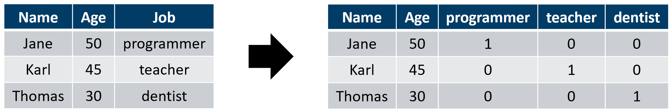
FIGURE 5.14: One-hot encoding example
Figure 5.15 presents a guideline for how to convert non-numeric variables into numeric ones for classification tasks. This is only a guideline and the actual process will depend on each application.
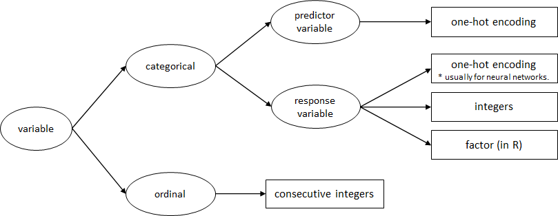
FIGURE 5.15: Variable conversion guidelines.
The caret package has a function dummyVars() that can be used to one-hot encode the categorical variables of a data frame. Since the STUDENTS’ MENTAL HEALTH dataset (Nguyen et al. 2019) has several categorical variables, it can be used to demonstrate how to apply dummyVars(). This dataset collected at a University in Japan contains survey responses from students about their mental health and help-seeking behaviors. We begin by loading the data.
# Load students mental health behavior dataset.
# stringsAsFactors is set to F since the function
# that we will use to one-hot encode expects characters.
dataset <- read.csv(file.path(datasets_path,
                              "students_mental_health",
                              "data.csv"),
                              stringsAsFactors = F)
Note that the stringsAsFactors parameter is set to FALSE. This is necessary because dummyVars() needs characters to work properly. Before one-hot encoding the variables, we need to do some preprocessing to clean the dataset. This dataset contains several fields with empty characters ‘““’. Thus, we will replace them with NA using the replace_with_na_all() function from the naniar package. This package was first described in the missing values section of this chapter, but that function was not mentioned. The function takes as its first argument the dataset and the second one is a formula that includes a condition.
# The dataset contains several empty strings.
# Replace those empty strings with NAs so the following
# methods will work properly.
# We can use the replace_with_na_all() function
# from naniar package to do the replacement.
library(naniar)
dataset <- replace_with_na_all(dataset,
                               ~.x %in% common_na_strings)
In this case, the condition is ~.x %in% common_na_strings which means: replace all fields that contain one of the characters in common_na_strings. The variable common_na_strings contains a set of common strings that can be regarded as missing values, for example ‘NA’, ‘na’, ‘NULL’, empty strings, and so on. Now, we can use the vis_miss() function described in the missing values section to get a visual idea of the missing values.
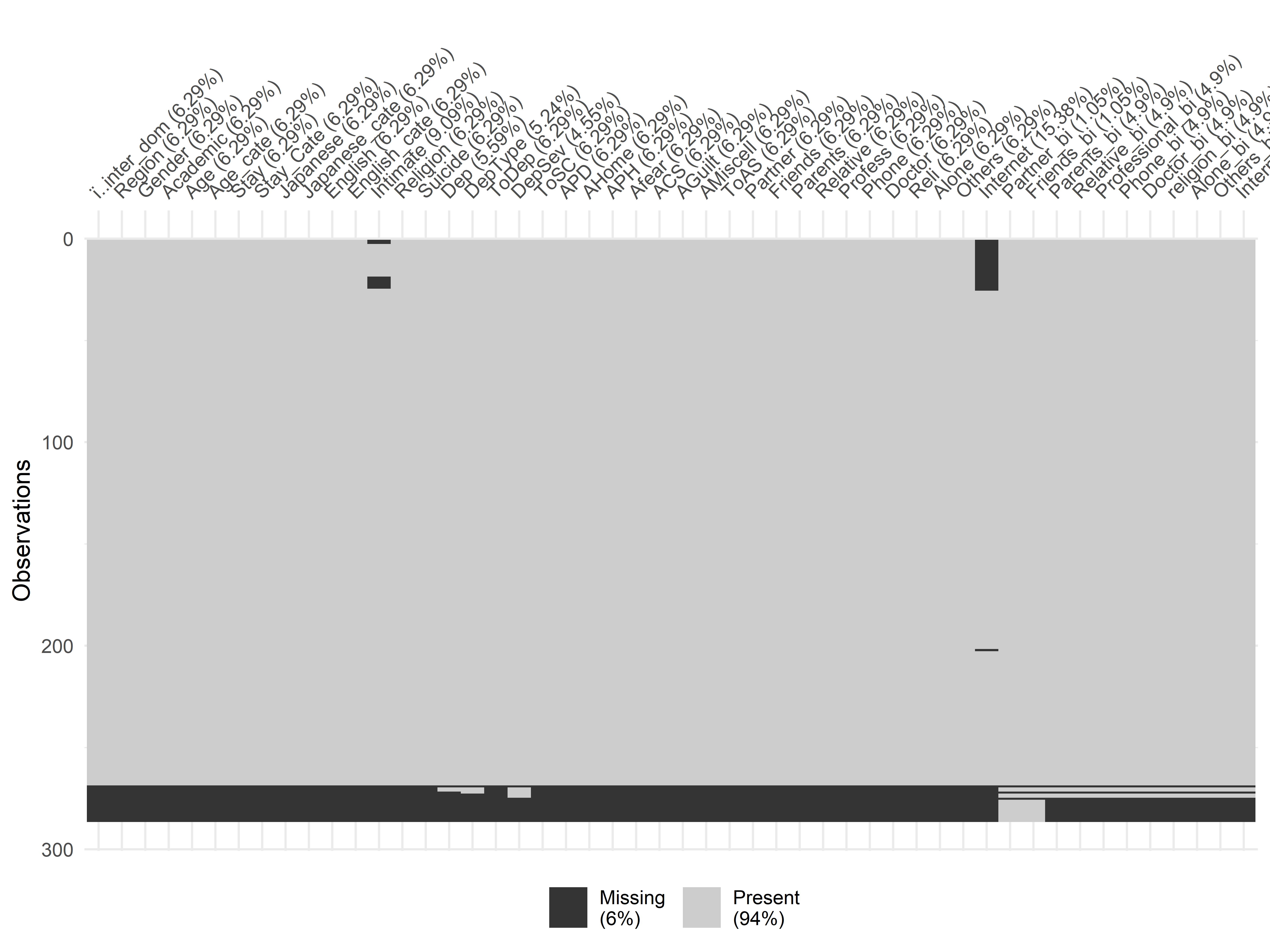
FIGURE 5.16: Missing values in the students mental health dataset.
Figure 5.16 shows the output plot. We can see that the last rows contain many missing values so we will discard them and only keep the first rows (\(1-268\)).
# Since the last rows starting at 269
# are full of missing values we will discard them.
dataset <- dataset[1:268,]
As an example, we will one-hot encode the Stay_Cate variable which represents how long a student has been at the university: 1 year (Short), 2–3 years (Medium), or at least 4 years (Long). The dummyVars() function takes a formula as its first argument. Here, we specify that we only want to convert Stay_Cate. This function does not do the actual encoding but returns an object that is used with predict() to obtain the encoded variable(s) as a new data frame.
# One-hot encode the Stay_Cate variable.
# This variable Stay_Cate has three possible
# values: Long, Short and Medium.
# First, create a dummyVars object with the dummyVars()
#function from caret package.
library(caret)

dummyObj <- dummyVars( ~ Stay_Cate, data = dataset)

# Perform the actual encoding using predict()
encodedVars <- data.frame(predict(dummyObj,
                                  newdata = dataset))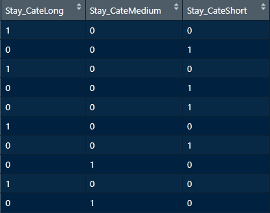
FIGURE 5.17: One-hot encoded Stay_Cate.
If we inspect the resulting data frame (Figure 5.17), we see that it has \(3\) variables, one for each possible value: Long, Medium, and Short. If this variable is used as a predictor variable, we should delete one of its columns to avoid the dummy variable trap. We can do this by setting the parameter fullRank = TRUE.
dummyObj <- dummyVars( ~ Stay_Cate, data = dataset, fullRank = TRUE)
encodedVars <- data.frame(predict(dummyObj, newdata = dataset))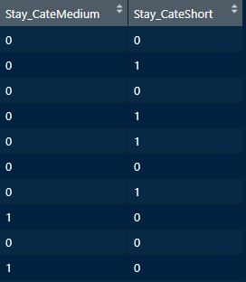
FIGURE 5.18: One-hot encoded Stay_Cate dropping one of the columns.
In this situation, the column with ‘Long’ was discarded (Figure 5.18). If you want to one-hot encode all variables at once you can use ~ . as the formula. But be aware that the dataset may have some categories encoded as numeric and thus will not be transformed. For example, the Age_cate encodes age categories but the categories are represented as integers from \(1\) to \(5\). In this case, it may be ok not to encode this variable since lower integer numbers also imply smaller ages and bigger integer numbers represent older ages. If you still want to encode this variable you could first convert it to character by appending a letter at the beginning. Sometimes you should encode a variable, for example, if it represents colors. In that situation, it does not make sense to leave it as numeric since there is not semantic order between colors.
5.7 Summary
Programming functions that train predictive models expect the data to be in a particular format. Furthermore, some methods make assumptions about the data like having no missing values, having all variables in the same scale, and so on. This chapter presented several commonly used methods to preprocess datasets before using them to train models.
- When collecting data from different sensors, we can face several sources of variation like sensors’ format, different sampling rates, different scales, and so on.
- Some preprocessing methods can lead to information injection. This happens when information from the train set is leaked to the test set.
- Missing values is a common problem in many data analysis tasks. In R, the
naniarpackage can be used to spot missing values. - Imputation is the process of inferring missing values. The
simputationpackage can be used to impute missing values in datasets. - Normalization is the process of transforming a set of variables to a common scale. For example from \(0\) to \(1\).
- An imbalanced dataset has a disproportionate number of classes of a certain type with respect to the others. Some methods like random over/under sampling and SMOTE can be used to balance a dataset.
- One-hot-encoding is a method that converts categorical variables into numeric ones.