Chapter 8 Predicting Behavior with Deep Learning
Deep learning (DL) consists of a set of model architectures and algorithms with applications in supervised, semi-supervised, unsupervised and reinforcement learning. Deep learning is mainly based on artificial neural networks (ANNs). One of the main characteristics of DL is that the models are composed of several levels. Each level transforms its input into more abstract representations. For example, for an image recognition task, the first level corresponds to raw pixels, the next level transforms pixels into simple shapes like horizontal/vertical lines, diagonals, etc. The next level may abstract more complex shapes like wheels, windows, and so on; and the final level could detect if the image contains a car or a human, or maybe both.
Examples of DL architectures include deep neural networks (DNNs), Convolutional Neural Networks (CNNs), recurrent neural networks (RNNs), and autoencoders, to name a few. One of the reasons of the success of DL is due to its flexibility to deal with different types of data and problems. For example, CNNs can be used for image classification, RNNs can be used for timeseries data, and autoencoders can be used to generate new data and perform anomaly detection. Another advantage of DL is that it is not always required to do feature engineering. That is, extract different features depending on the problem domain. Depending on the problem and the DL architecture, it is possible to feed the raw data (with some preprocessing) to the model. The model will then, automatically extract features at each level with an increasing level of abstraction. DL has achieved state-of-the-art results in many different tasks including speech recognition, image recognition, and translation. It has also been successfully applied to different types of behavior prediction.
In this chapter, an introduction to artificial neural networks will be presented. Next, I will explain how to train deep models in R using Keras and TensorFlow. The models will be applied to behavior prediction tasks. This chapter also includes a section on Convolutional Neural Networks and their application to behavior prediction.
8.1 Introduction to Artificial Neural Networks
Artificial neural networks (ANNs) are mathematical models inspired by the brain. Here, I would like to emphasize the word inspired because ANNs do not model how a biological brain actually works. In fact, there is little knowledge about how a biological brain works. ANNs are composed of units (also called neurons or nodes) and connections between units. Each unit can receive inputs from other units. Those inputs are processed inside the unit and produce an output. Typically, units are arranged into layers (as we will see later) and connections between units have an associated weight. Those weights are learned during training and they are the core elements that make a network behave in a certain way.
Before going into details of how multi-layer ANNs work, let’s start with a very simple neural network consisting of a single unit. See Figure 8.1. Even though this network only has one node, it is already composed of several interesting elements which are the basis of more complex networks. First, it has \(n\) input variables \(x_1 \ldots x_n\) which are real numbers. Second, the unit has a set of \(n\) weights \(w_1 \ldots w_n\) associated with each input. These weights can take real numbers as values. Finally, there is an output \(y'\) which is binary (it can take two values: \(1\) or \(0\)).
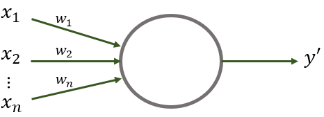
FIGURE 8.1: A neural network composed of a single unit (perceptron).
This single unit also known as perceptron is capable of making binary decisions based on the input and the weights. To get the final decision \(y'\) the inputs are multiplied by their corresponding weights and the results are summed. If the sum is greater than a given threshold, then the output is \(1\) and \(0\) otherwise. Formally:
\[\begin{equation} y' = \begin{cases} 1 & \textit{if } \sum_{i}{w_i x_i > t}, \\ 0 & \textit{if } \sum_{i}{w_i x_i \leq t} \end{cases} \tag{8.1} \end{equation}\]
where \(t\) is a threshold. We can use a perceptron to make important decisions in life. For example, suppose you need to decide whether or not to go to the movies. Assume this decision is based on two pieces of information:
- You have money to pay the entrance (or not) and,
- it is a horror movie (or not).
There are two additional assumptions as well:
- The movie theater only projects \(1\) film.
- You don’t like horror movies.
This decision-making process can be modeled with the perceptron of Figure 8.2. This perceptron has two binary input variables: money and horror. Each variable has an associated weight. Suppose there is a decision threshold of \(t=3\). Finally, there is a binary output: \(1\) means you should go to the movies and \(0\) indicates that you should not go.
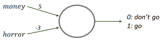
FIGURE 8.2: Perceptron to decide whether or not to go to the movies based on two input variables.
Suppose that today was payday and the theater is projecting an action movie. Then, we can set the input variables \(money=1\) and \(horror=0\). Now we want to decide if we should go to the movie theater or not. To get the final answer we can use Equation (8.1). This formula tells us that we need to multiply each input variable with their corresponding weights and add them:
\[\begin{align*} (money)(5) + (horror)(-3) \end{align*}\]
Substituting money and horror with their corresponding values:
\[\begin{align*} (1)(5) + (0)(-3) = 5 \end{align*}\]
Since \(5 > t\) (remember the threshold \(t=3\)), the final output will be \(1\), thus, the advice is to go to the movies. Let’s try the scenario when you have money but they are projecting a horror movie: \(money=1\), \(horror=1\).
\[\begin{align*} (1)(5) + (1)(-3) = 2 \end{align*}\]
In this case, \(2 < t\) and the final output is \(0\). Even if you have money, you should not waste it on a movie that you know you most likely will not like. This process of applying operations to the inputs and obtaining the final result is called forward propagation because the inputs are ‘pushed’ all the way through the network (a single perceptron in this case). For bigger networks, the outputs of the current layer become the inputs of the next layer, and so on.
For convenience, a simplified version of Equation (8.1) can be used. This alternative representation is useful because it provides flexibility to change the internals of the units (neurons) as we will see. The first simplification consists of representing the inputs and weights as vectors:
\[\begin{equation} \sum_{i}{w_i x_i} = \boldsymbol{w} \cdot \boldsymbol{x} \end{equation}\]
The summation becomes a dot product between \(\boldsymbol{w}\) and \(\boldsymbol{x}\). Next, the threshold \(t\) can be moved to the left and renamed to \(b\) which stands for bias. This is only for notation but you can still think of the bias as a threshold.
\[\begin{equation} y' = f(\boldsymbol{x}) = \begin{cases} 1 & \textit{if } \boldsymbol{w} \cdot \boldsymbol{x} + b > 0, \\ 0 & \textit{otherwise} \end{cases} \end{equation}\]
The output \(y'\) is a function of \(\boldsymbol{x}\) with \(\boldsymbol{w}\) and \(b\) as fixed parameters. One thing to note is that first, we are performing the operation \(\boldsymbol{w} \cdot \boldsymbol{x} + b\) and then, another operation is applied to the result. In this case, it is a comparison. If the result is greater than \(0\) the final output is \(1\). You can think of this second operation as another function. Call it \(g(x)\).
\[\begin{equation} f(\boldsymbol{x}) = g(\boldsymbol{w} \cdot \boldsymbol{x} + b) \tag{8.2} \end{equation}\]
In neural networks terminology, this \(g(x)\) is known as the activation function. Its result indicates how much active this unit is based on its inputs. If the result is \(1\), it means that this unit is active. If the result is \(0\), it means the unit is inactive.
This new notation allows us to use different activation functions by substituting \(g(x)\) with some other function in Equation (8.2). In the case of the perceptron, the activation function \(g(x)\) is the threshold function, which is known as the step function:
\[\begin{equation} g(x) = step(x) = \begin{cases} 1 & \textit{if } x > 0 \\ 0 & \textit{if } x \leq 0 \end{cases} \tag{8.3} \end{equation}\]
Figure 8.3 shows the plot of the step function.
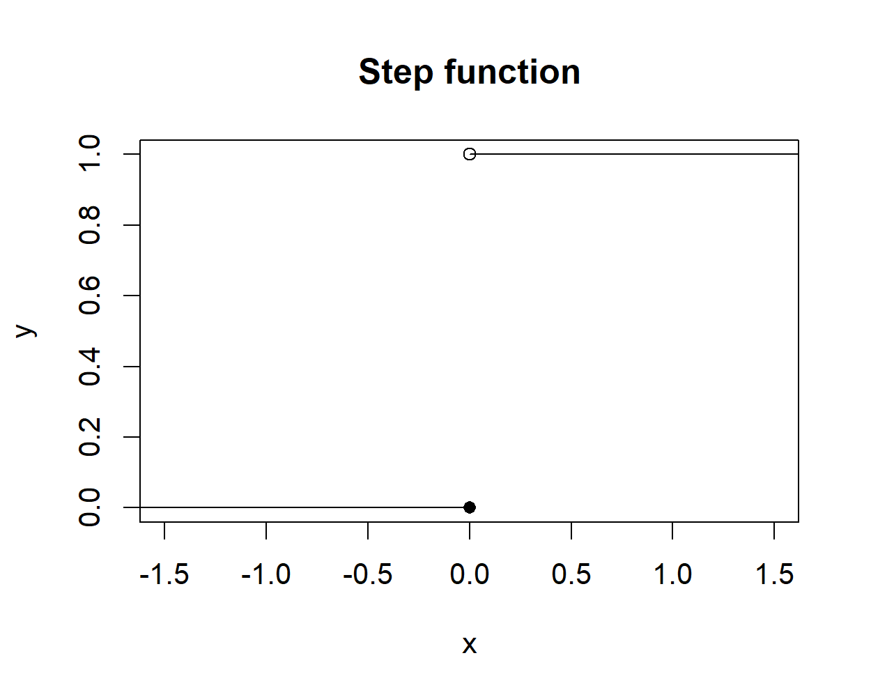
FIGURE 8.3: The step function.
It is worth noting that perceptrons have two major limitations:
- The output is binary.
- Perceptrons are linear functions.
The first limitation imposes some restrictions on its applicability. For example, a perceptron cannot be used to predict real-valued outputs which is a fundamental aspect for regression problems. The second limitation makes the perceptron only capable of solving linear problems. Figure 8.4 graphically shows this limitation. In the first case, the outputs of the OR logical operator can be classified (separated) using a line. On the other hand, it is not possible to classify the output of the XOR function using a single line.
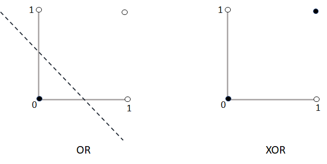
FIGURE 8.4: The OR and the XOR logical operators.
To overcome those limitations, several modifications to the perceptron were introduced. This allows us to build models capable of solving more complex non-linear problems. One such modification is to change the activation function. Another improvement is to add the ability to have several layers of interconnected units. In the next section, two new types of units will be presented. Then, the following section will introduce neural networks also known as multilayer perceptrons which are more complex models built by connecting many units and arranging them into layers.
8.1.1 Sigmoid and ReLU Units
As previously mentioned, perceptrons have some limitations that restrict their applicability including the fact that they are linear models. In practice, problems are complex and most of them are non-linear. One way to overcome this limitation is to introduce non-linearities and this can be done by using a different type of activation function. Remember that a unit can be modeled as \(f(x) = g(wx+b)\) where \(g(x)\) is some activation function. For the perceptron, \(g(x)\) is the step function. However, another practical limitation not mentioned before is that the step function can change abruptly from \(0\) to \(1\) and vice versa. Small changes in \(x\), \(w\), or \(b\) can completely change the output. This is a problem during learning and inference time. Instead, we would prefer a smooth version of the step function, for example, the sigmoid function which is also known as the logistic function:
\[\begin{equation} s(x) = \frac{1}{1 + e^{-x}} \tag{8.4} \end{equation}\]
This function has an ‘S’ shape (Figure 8.5) and as opposed to a step function, this one is smooth. The range of this function is from \(0\) to \(1\).
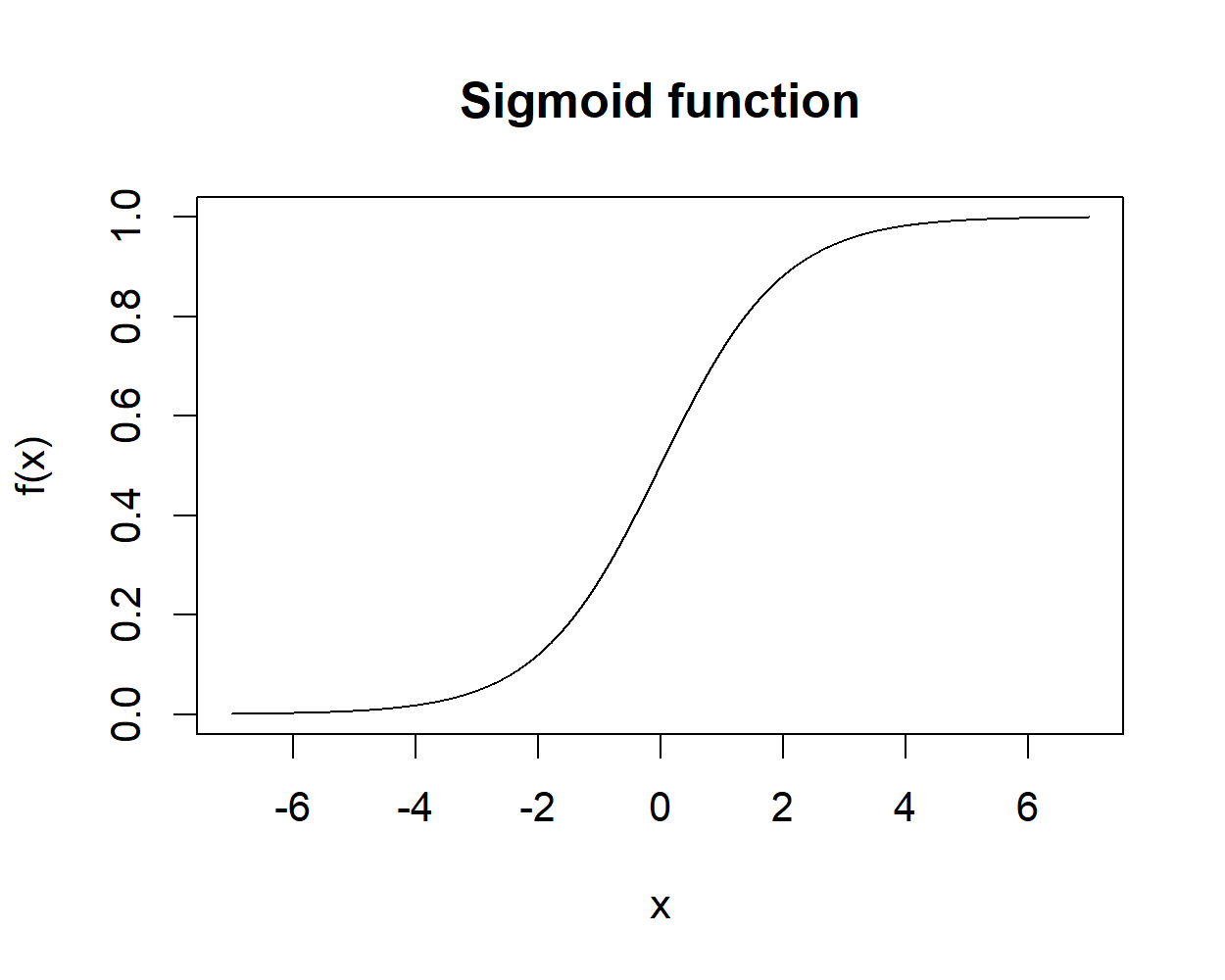
FIGURE 8.5: Sigmoid function.
If we substitute the activation function in Equation (8.2) with the sigmoid function we get our sigmoid unit:
\[\begin{equation} f(x) = \frac{1}{1 + e^{-(w \cdot x + b)}} \tag{8.5} \end{equation}\]
Sigmoid units have been one of the most commonly used types of units when building bigger neural networks. Another advantage is that the outputs are real values that can be interpreted as probabilities. For instance, if we want to make binary decisions we can set a threshold. For example, if the output of the sigmoid unit is \(> 0.5\) then return a \(1\). Of course, that threshold would depend on the application. If we need more confidence about the result we can set a higher threshold.
In the last years, another type of unit has been successfully applied to train neural networks, the rectified linear unit or ReLU for short (Figure 8.6).
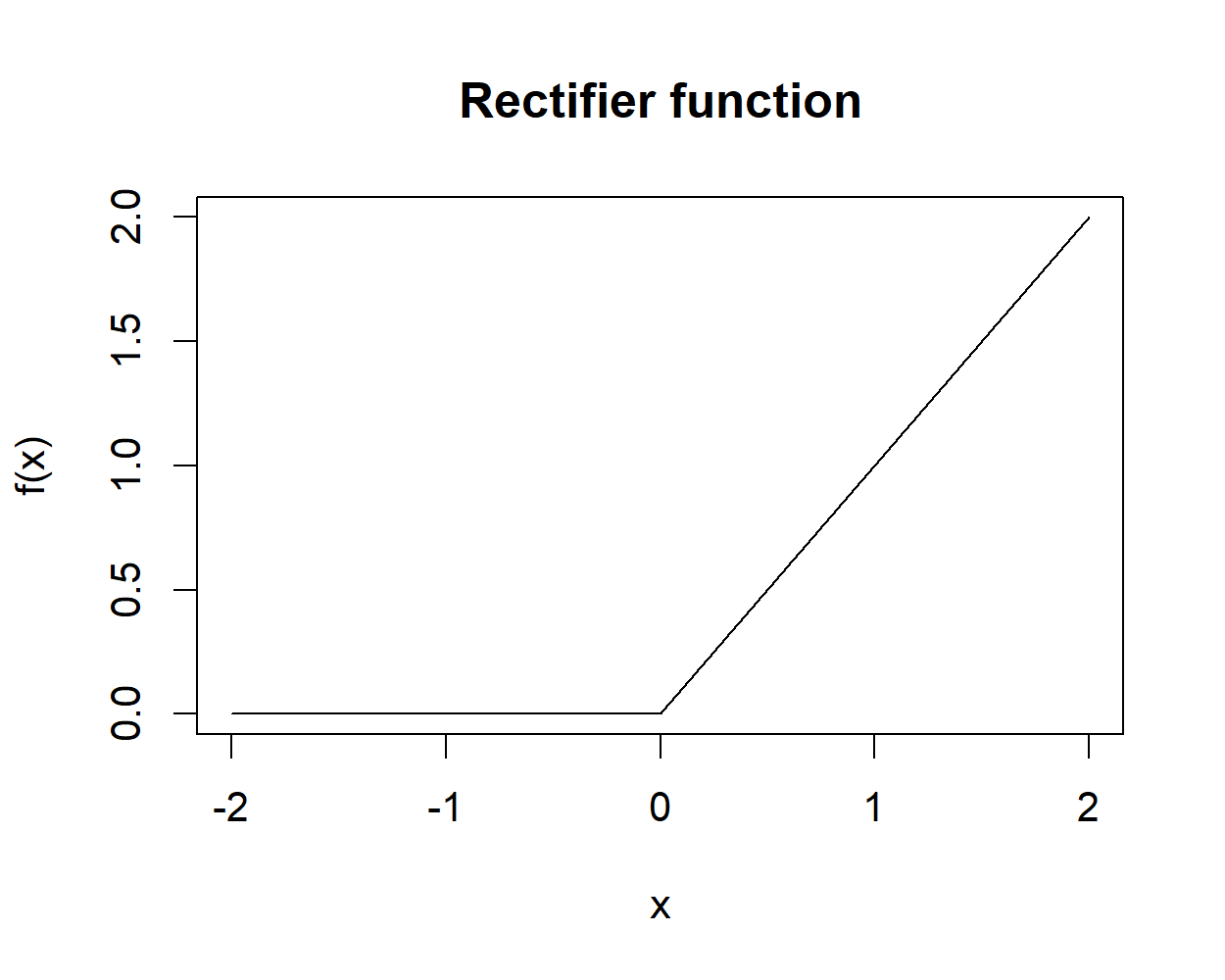
FIGURE 8.6: Rectifier function.
The activation function of this unit is the rectifier function:
\[\begin{equation} rectifier(x) = \begin{cases} 0 & \textit{if } x < 0, \\ x & \textit{if } x \geq 0 \end{cases} \tag{8.6} \end{equation}\]
This one is also called the ramp function and is one of the simplest non-linear functions and probably the most common one used in modern big neural networks. These units present several advantages, being among them, efficiency during training and inference time.
So far, we have been talking about single units. In the next section, we will see how these single units can be assembled to build bigger artificial neural networks.
8.1.2 Assembling Units into Layers
Perceptrons, sigmoid, and ReLU units can be thought of as very simple neural networks. By connecting several units, one can build more complex neural networks. For historical reasons, neural networks are also called multilayer perceptrons regardless whether the units are perceptrons or not. Typically, units are grouped into layers. Figure 8.7 shows an example neural network with \(3\) layers. An input layer with \(3\) nodes, a hidden layer with \(2\) nodes, and an output layer with \(1\) node.
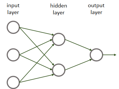
FIGURE 8.7: Example neural network.
This network only has one hidden layer. Hidden layers are called like that because they do not have direct contact with the external world. Finally, there is an output layer with a single unit. We could also have an output layer with more than one unit. Most of the time, we will have fully connected neural networks. That is, all units have incoming connections from all nodes in the previous layer (as in the previous example).
We already saw how a unit can produce a result based on the inputs by using forward propagation. For more complex networks the process is the same! Consider the network shown in Figure 8.8. It consists of two inputs and one output. It also has one hidden layer with \(2\) units.
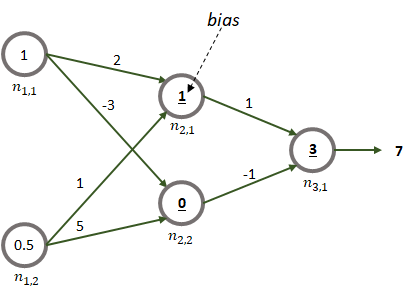
FIGURE 8.8: Example of forward propagation.
Each node is labeled as \(n_{l,n}\) where \(l\) is the layer and \(n\) is the unit number. The two input values are \(1\) and \(0.5\). They could be temperature measurements, for example. Each edge has an associated weight. For simplicity, let’s assume that the activation function of the units is the identity function \(g(x)=x\). The bold underlined number inside the nodes of the hidden and output layers are the biases. Here we assume that the network is already trained (later we will see how those weights and biases are learned). To get the final result, for each node, its inputs are multiplied by their corresponding weights and added. Then, the bias is added. Next, the activation function is applied. In this case, it is just the identify function (returns the same value). The outputs of the nodes in the hidden layer become the inputs of the next layer and so on.
In this example, first we need to compute the outputs of nodes \(n_{2,1}\) and \(n_{2,2}\):
output of \(n_{2,1} = (1)(2) + (0.5)(1) + 1 = 3.5\)
output of \(n_{2,2} = (1)(-3) + (0.5)(5) + 0 = -0.5\)
Finally, we can compute the output of the last node using the outputs of the previous nodes:
output of \(n_{3,1} = (3.5)(1) + (-0.5)(-1) + 3 = 7\).
8.1.3 Deep Neural Networks
By increasing the number of layers and the number of units in each layer, one can build more complex networks. But what is a deep neural network (DNN)? There is not a strict rule but some people say that a network with more than \(2\) hidden layers is a deep network. Yes, that’s all it takes to build a DNN! Figure 8.9 shows an example of a deep neural network.
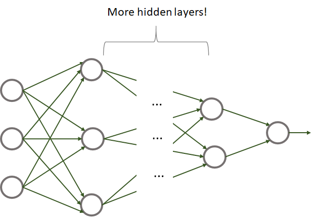
FIGURE 8.9: Example of a deep neural network.
A DNN has nothing special compared to a traditional neural network except that it has many layers. One of the reasons why they became so popular until recent years is because before, it was not possible to efficiently train them. With the advent of specialized hardware like graphics processing units (GPUs), it is now possible to efficiently train big DNNs. The introduction of ReLU units was also a key factor that allowed the training of even bigger networks. The availability of big quantities of data was another key factor that allowed the development of deep learning technologies. Note that deep learning is not limited to DNNs but it also encompasses other types of architectures like convolutional networks and recurrent neural networks, to name a few. Convolutional layers will be covered later in this chapter.
8.1.4 Learning the Parameters
We have seen how forward propagation can be used at inference time to compute the output of the network based on the input values. In the previous examples, we assumed that the network’s parameters (weights and biases) were already learned. In practice, you most likely will use libraries and frameworks to build and train neural networks. Later in this chapter, I will show you how to use TensorFlow and Keras within R. But, before that, I will explain how the networks’ parameters are learned and how to code and train a very simple network from scratch.
Back to the problem, the objective is to find the parameters’ values based on training data such that the predicted result for any input data point is as close as possible as the true value. Put in other words, we want to find the parameters’ values that reduce the network’s prediction error.
One way to estimate the network’s error is by computing the squared difference between the prediction \(y'\) and the real value \(y\), that is, \(error = (y' - y)^2\). This is how the error can be computed for a single training data point. The error function is typically called the loss function and denoted by \(L(\theta)\) where \(\theta\) represents the parameters of the network (weights and biases). In this example the loss function is \(L(\theta)=(y'- y)^2\).
If there is more than one training data point (which is often the case), the loss function is just the average of the individual squared differences which is known as the mean squared error (MSE):
\[\begin{equation} L(\theta) = \frac{1}{N} \sum_{n=1}^N{(y'_n - y_n)^2} \tag{8.7} \end{equation}\]
The problem of finding the best parameters can be formulated as an optimization problem, that is, find the optimal parameters such that the loss function is minimized. This is the learning/training phase of a neural network. Formally, this can be stated as:
\[\begin{equation} \operatorname*{arg min}_{\theta} L(\theta) \tag{8.8} \end{equation}\]
This notation means: find and return the weights and biases that make the loss function be as small as possible.
The most common method to train neural networks is called gradient descent. The algorithm updates the parameters in an iterative fashion based on the loss. This algorithm is suitable for complex functions with millions of parameters.
Suppose there is a network with only \(1\) weight and no bias with MSE as loss function (Equation (8.7)). Figure 8.10 shows a plot of the loss function. This is a quadratic function that only depends on the value of \(w\). The task is to find the \(w\) where the function is at its minimum.
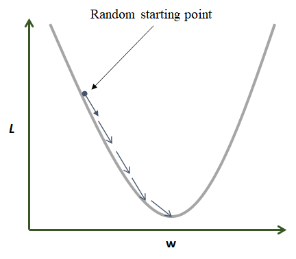
FIGURE 8.10: Gradient descent in action.
Gradient descent starts by assigning \(w\) a random value. Then, at each step and based on the error, \(w\) is updated in the direction that minimizes the loss function. In the previous figure, the global minimum is found after \(5\) iterations. In practice, loss functions are more complex and have many local minima (Figure 8.11). For complex functions, it is difficult to find a global minimum but gradient descent can find a local minimum that is good enough to solve the problem at hand.
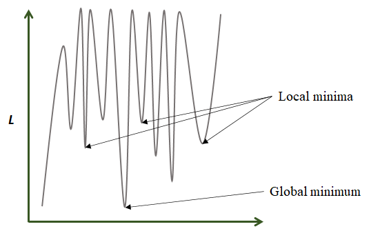
FIGURE 8.11: Function with 1 global minimum and several local minima.
But in what direction and how much is \(w\) moved in each iteration? The direction and magnitude are estimated by computing the derivative of the loss function with respect to the weight \(\frac{\partial L}{\partial w}\). The derivative is also called the gradient and denoted by \(\nabla L\). The iterative gradient descent procedure is listed below:
for each \(w_i\) in \(W\) do:
\(w_i = w_i - \alpha \frac{\partial L(W)}{\partial w_i}\)
The outer loop is run until the algorithm converges or until a predefined number of iterations is reached. Each iteration is also called an epoch. Each weight is updated with the rule: \(w_i = w_i - \alpha \frac{\partial L(W)}{\partial w_i}\). The derivative part will give us the direction and magnitude. The \(\alpha\) is called the learning rate and it controls how ‘fast’ we move. The learning rate is a constant defined by the user, thus, it is a hyperparameter. A high learning rate can cause the algorithm to miss the local minima and the loss can start to increase. A small learning rate will cause the algorithm to take more time to converge. Figure 8.12 illustrates both scenarios.
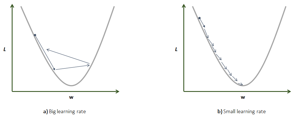
FIGURE 8.12: Comparison between high and low learning rates. a) Big learning rate. b) Small learning rate.
Selecting an appropriate learning rate will depend on the application but common values are between \(0.0001\) and \(0.05\).
Let’s see how gradient descent works with a step by step example. Consider a very simple neural network consisting of an input layer with only one input feature and an output layer with one unit and no bias. To make it even simpler, the activation function of the output unit is the identity function \(f(x)=x\). Assume that as training data we have a single data point. Figure 8.13 shows the simple network and the training data. The training data point only has one input variable (\(x\)) and an output (\(y\)). We want to train this network such that it can make predictions on new data points. The training point has an input feature of \(x=3\) and the expected output is \(y=1.5\). For this particular training point, it seems that the output is equal to the input divided by \(2\). Thus, based on this single training data point the network should learn how to divide any other input by \(2\).
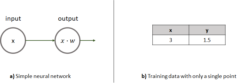
FIGURE 8.13: a) A simple neural network consisting of one unit. b) The training data with only one row.
Before we start the training we need to define \(3\) things:
The loss function. This is a regression problem so we can use the MSE. Since there is a single data point our loss function becomes \(L(w)=(y' - y)^2\). Here, \(y\) is the ground truth output value and \(y'\) is the predicted value. We know how to make predictions using forward propagation. In this case, it is the product between the input value and the single weight, and the activation function has no effect (it returns the same value as its input). We can rewrite the loss function as \(L(w)=(xw - y)^2\).
We need to define a learning rate. For now, we can set it to \(\alpha = 0.05\).
The weights need to be initialized at random. Let’s assume the single weight is ‘randomly’ initialized with \(w=2\).
Now we can use gradient descent to iteratively update the weight. Remember that the updating rule is:
\[\begin{equation} w = w - \alpha \frac{\partial L(w)}{\partial w} \end{equation}\]
The partial derivative of the loss function with respect to \(w\) is:
\[\begin{equation} \frac{\partial L(w)}{\partial w} = 2x(xw - y) \end{equation}\]
If we substitute the derivative in the updating rule we get:
\[\begin{equation} w = w - \alpha 2x(xw - y) \end{equation}\]
We already know that \(\alpha=0.05\), the input value is \(x=3\), the output is \(y=1.5\) and the initial weight is \(w=2\). So we can start updating \(w\). Figure 8.14 shows the initial state (iteration 0) and \(3\) additional iterations. In the initial state, \(w=2\) and with that weight the loss is \(20.25\). In iteration \(1\), the weight is updated and now its value is \(0.65\). With this new weight, the loss is \(0.2025\). That was a substantial reduction in the error! After three iterations we see that the final weight is \(w=0.501\) and the loss is very close to zero.
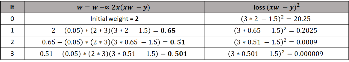
FIGURE 8.14: First 3 gradient descent iterations (epochs).
Now, we can start doing predictions with our very simple neural network! To do so, we use forward propagation on the new input data using the learned weight \(w=0.501\). Figure 8.15 shows the predictions on new training data points that were never seen before by the network.
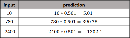
FIGURE 8.15: Example predictions on new data points.
Even though the predictions are not perfect, they are very close to the expected value (division by \(2\)) considering that the network is very simple and was only trained with a single data point and for only \(3\) epochs!
If the training set has more than one data point, then we need to compute the derivative of each point and accumulate them (the derivative of a sum is equal to the sum of the derivatives). In the previous example, the update rule becomes:
\[\begin{equation} w = w - \alpha \sum_{i=1}^N{2x_i(x_i w - y)} \end{equation}\]
This means that before updating a weight, first, we need to compute the derivative for each point and add them. This needs to be done for every parameter in the network. Thus, one epoch is a pass through all training points and all parameters.
8.1.5 Parameter Learning Example in R
gradient_descent.R
In the previous section, we went step by step to train a neural network with a single unit and with a single training data point. Here, we will see how we can implement that simple network in R but when we have more training data. The code can be found in the script gradient_descent.R.
This code implements the same network as the previous example. That is, one neuron, one input, no bias, and activation function \(f(x) = x\). We start by creating a sample training set with \(3\) points. Again, the output is the input divided by \(2\).
train_set <- data.frame(x = c(3.0,4.0,1.0), y = c(1.5, 2.0, 0.5))
# Print the train set.
print(train_set)
#>   x   y
#> 1 3 1.5
#> 2 4 2.0
#> 3 1 0.5
Then we need to implement three functions: forward propagation, the loss function, and the derivative of the loss function.
# Forward propagation w*x
fp <- function(w, x){
    return(w * x)
}

# Loss function (y - y')^2
loss <- function(w, x, y){
  predicted <- fp(w, x) # This is y'
  return((y - predicted)^2)
}

# Derivative of the loss function. 2x(xw - y)
derivative <- function(w, x, y){
  return(2.0 * x * ((x * w) - y))
}
Now we are all set to implement the gradient.descent() function. The first parameter is the train set, the second parameter is the learning rate \(\alpha\), and the last parameter is the number of epochs. The initial weight is initialized to some ‘random’ number (selected manually here for the sake of the example). The function returns the final learned weight.
# Gradient descent.
gradient.descent <- function(train_set, lr = 0.01, epochs = 5){

  w = -2.5 # Initialize weight at 'random'

  for(i in 1:epochs){
    derivative.sum <- 0.0
    loss.sum <- 0.0

    # Iterate each data point in train_set.
    for(j in 1:nrow(train_set)){
      point <- train_set[j, ]

      derivative.sum <- derivative.sum + derivative(w, point$x, point$y)

      loss.sum <- loss.sum + loss(w, point$x, point$y)
    }

    # Update weight.
    w <-  w - lr * derivative.sum

    # mean squared error (MSE)
    mse <- loss.sum / nrow(train_set)

    print(paste0("epoch: ", i, " loss: ",
                 formatC(mse, digits = 8, format = "f"),
                 " w = ", formatC(w, digits = 5, format = "f")))
  }

  return(w)
}
Now, let’s train the network with a learning rate of \(0.01\) and for \(10\) epochs. This function will print for each epoch, the loss and the current weight.
#### Train the 1 unit network with gradient descent ####
lr <- 0.01 # set learning rate.

set.seed(123)

# Run gradient decent to find the optimal weight.
learned_w = gradient.descent(train_set, lr, epochs = 10)

#> [1] "epoch: 1 loss: 78.00000000 w = -0.94000"
#> [1] "epoch: 2 loss: 17.97120000 w = -0.19120"
#> [1] "epoch: 3 loss: 4.14056448 w = 0.16822"
#> [1] "epoch: 4 loss: 0.95398606 w = 0.34075"
#> [1] "epoch: 5 loss: 0.21979839 w = 0.42356"
#> [1] "epoch: 6 loss: 0.05064155 w = 0.46331"
#> [1] "epoch: 7 loss: 0.01166781 w = 0.48239"
#> [1] "epoch: 8 loss: 0.00268826 w = 0.49155"
#> [1] "epoch: 9 loss: 0.00061938 w = 0.49594"
#> [1] "epoch: 10 loss: 0.00014270 w = 0.49805"
From the output, we can see that the loss decreases as the weight is updated. The final value of the weight at iteration \(10\) is \(0.49805\). We can now make predictions on new data.
# Make predictions on new data using the learned weight.
fp(learned_w, 7)
#> [1] 3.486366

fp(learned_w, -88)
#> [1] -43.8286
Now, you can try to change the training set to make the network learn a different arithmetic operation!
In the previous example, we considered a very simple neural network consisting of a single unit. In this case, the partial derivative with respect to the single weight was calculated directly. For bigger networks with more layers and activations, the final output becomes a composition of functions. That is, the activation values of a layer \(l\) depend on its weights which are also affected by the previous layer’s \(l-1\) weights and so on. So, the derivatives (gradients) can be computed using the chain rule \(f(g(x))' = f'(g(x)) \cdot g'(x)\). This can be performed efficiently by an algorithm known as backpropagation.
“What backpropagation actually lets us do is compute the partial derivatives \(\partial C_x / \partial w\) and \(\partial C_x / \partial b\) for a single training example”. (Michael Nielsen, 2019)20.
Here, \(C\) refers to the loss function which is also called the cost function. In modern deep learning libraries like TensorFlow, this procedure is efficiently implemented with a computational graph. If you want to learn the details about backpropagation I recommend you to check this post by DEEPLIZARD (https://deeplizard.com/learn/video/XE3krf3CQls) which consists of \(5\) parts including videos.
8.1.6 Stochastic Gradient Descent
We have seen how gradient descent iterates over all training points before updating each parameter. To recall, an epoch is one pass through all parameters and for each parameter, the derivative with each training point needs to be computed. If the training set consists of thousands or millions of points, this method becomes very time-consuming. Furthermore, in practice neural networks do not have one or two parameters but thousands or millions. In those cases, the training can be done more efficiently by using stochastic gradient descent (SGD). This method adds two main modifications to the classic gradient descent:
- At the beginning, the training set is shuffled (this is the stochastic part). This is necessary for the method to work.
- The training set is divided into \(b\) batches with \(m\) data points each. This \(m\) is known as the batch size and is a hyperparameter that we need to define.
Then, at each epoch all batches are iterated and the parameters are updated based on each batch and not the entire training set, for example:
\[\begin{equation} w = w - \alpha \sum_{i=1}^m{2x_i(x_i w - y)} \end{equation}\]
Again, an epoch is one pass through all parameters and all batches. Now you may be wondering why this method is more efficient if an epoch still involves the same number of operations but they are split into chunks. Part of this is because since the parameter updates are more frequent, the loss also improves quicker. Another reason is that the operations within each batch can be optimized and performed in parallel, for example, by using a GPU. One thing to note is that each update is based on less information by only using \(m\) points instead of the entire data set. This can introduce some noise in the learning but at the same time this can help to get out of local minima. In practice, SGD needs more epochs to converge compared to gradient descent but overall, it will take less time. From now on, this is the method we will use to train our networks.
8.2 Keras and TensorFlow with R
TensorFlow21 is an open-source computational library used mainly for machine learning and more specifically, for deep learning. It has many available tools and extensions to perform a wide variety of tasks such as data pre-processing, model optimization, reinforcement learning, probabilistic reasoning, to name a few. TensorFlow is very flexible and is used for research, development, and in production environments. It provides an API that contains the necessary building blocks to build different types of neural networks including CNNs, autoencoders, Recurrent Neural Networks, etc. It has two main versions. A CPU version and a GPU version. The latter allows the execution of programs by taking advantage of the computational power of graphic processing units. This makes training models much faster. Despite all this flexibility and power, it can take some time to learn the basics. Sometimes you need a way to build and test machine learning models in a simple way, for example, when trying new ideas or prototyping. Fortunately, there exists an interface to TensorFlow called Keras22.
Keras offers an API that abstracts many of the TensorFlow’s details making it easier to build and train machine learning models. Keras is what I will use when building deep learning models in this book. Keras does not only provide an interface to TensorFlow but also to other deep learning engines such as Theano23, Microsoft Cognitive Toolkit24, etc. Keras was developed by François Chollet and later, it was integrated with TensorFlow.
Most of the time its API should be enough to do common tasks and it provides ways to add extensions in case that is not enough. In this book, we will only use a subset of the available Keras functions but that will be enough for our purposes of building models to predict behaviors. If you want to learn more about Keras, I recommend the book “Deep Learning with R” by Chollet and Allaire (2018).
Examples in this book will use Keras with TensorFlow as the backend. In R, we can access Keras through the keras package (Allaire and Chollet 2019).
In the next section, we will start with a simple model built with Keras and the following examples will introduce more functions. By the end of this chapter you will be able to build and train efficient deep neural networks including Convolutional Neural Networks.
8.2.1 Keras Example
keras_simple_network.R
If you haven’t already installed Keras and TensorFlow, I would recommend you to do so at this point. Instructions on how to install the required software can be found in Appendix A.
In the previous section, I showed how to implement gradient descent in R (see gradient_descent.R). Now, I will show how to implement the same simple network using Keras. Recall that our network has one unit, one input, one output, and no bias. The code can be found in the script keras_simple_network.R. First, the keras library is loaded and a sample training set is created. Then, the function keras_model_sequential() is used to instantiate a new empty model. It is called sequential because it consists of a sequence of layers. At this point it does not have any layers yet.
library(keras)

# Generate a train set.
# First element is the input x and
# the second element is the output y.
train_set <- data.frame(x = c(3.0,4.0,1.0),
                        y = c(1.5, 2.0, 0.5))

# Instantiate a sequential model.
model <- keras_model_sequential()
We can now start adding layers (only one in this example). To do so, the layer_dense() method can be used. The dense name means that this will be a densely (fully) connected layer. This layer will be the output layer with a single unit.
The first argument units = 1 specifies the number of units in this layer. By default, a bias is added in each layer. To make it the same as in the previous example, we will not use a bias so use_bias is set to FALSE. The activation specifies the activation function. Here it is set to 'linear' which means that no activation function is applied \(f(x)=x\). Finally, we need to specify the number of inputs with input_shape. In this case, there is only one feature.
Before training the network we need to compile the model and specify the learning algorithm. In this case, stochastic gradient descent with a learning rate of \(\alpha=0.01\). We also need to specify which loss function to use (we’ll use mean squared error). At every epoch, some performance metrics can be computed. Here, we specify that we want the mean squared error and mean absolute error. These metrics are computed on the train data. After compiling the model, the summary() method can be used to print a textual description of it. Figure 8.16 shows the output of the summary() function.
model %>% compile(
  optimizer = optimizer_sgd(lr = 0.01),
  loss = 'mse',
  metrics = list('mse','mae')
)
summary(model)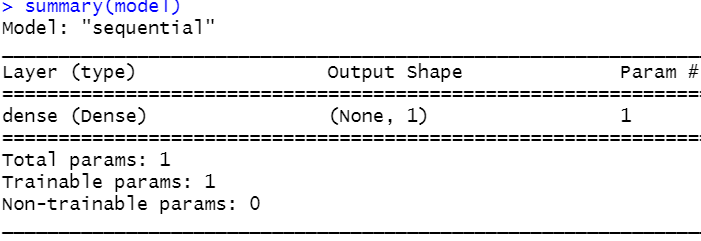
FIGURE 8.16: Summary of the simple neural network.
From this output, we see that the network consists of a single dense layer with \(1\) unit.
To start the actual training procedure we need to call the fit() function. Its first argument is the input training data (features) as a matrix. The second argument specifies the corresponding true outputs. We let the algorithm run for \(30\) epochs. The batch size is set to \(3\) which is also the total number of data points in our data. In this example the dataset is very small so we set the batch size equal to the total number of instances. In practice, datasets can contain thousands of instances but the batch size will be relatively small (e.g., \(8\), \(16\), \(32\), etc.).
Additionally, there is a validation_split parameter that specifies the fraction of the train data to be used for validation. This is set to \(0\) (the default) since the dataset is very small. If the validation split is greater than \(0\), its performance metrics will also be computed. The verbose parameter sets the amount of information to be printed during training. A \(0\) will not print anything. A \(2\) will print one line of information per epoch. The last parameter view_metrics specifies if you want the progress of the loss and performance metrics to be plotted. The fit() function returns an object with summary statistics collected during training and is saved in the variable history.
history <- model %>% fit(
  as.matrix(train_set$x), as.matrix(train_set$y),
  epochs = 30,
  batch_size = 3,
  validation_split = 0,
  verbose = 2,
  view_metrics = TRUE
)
Figure 8.17 presents the output of the fit() function in RStudio. In the console, the training loss, mean squared error, and mean absolute error are printed during each epoch. In the viewer pane, plots of the same metrics are shown. Here, we can see that the loss is nicely decreasing over time. The loss at epoch \(30\) should be close to \(0\).
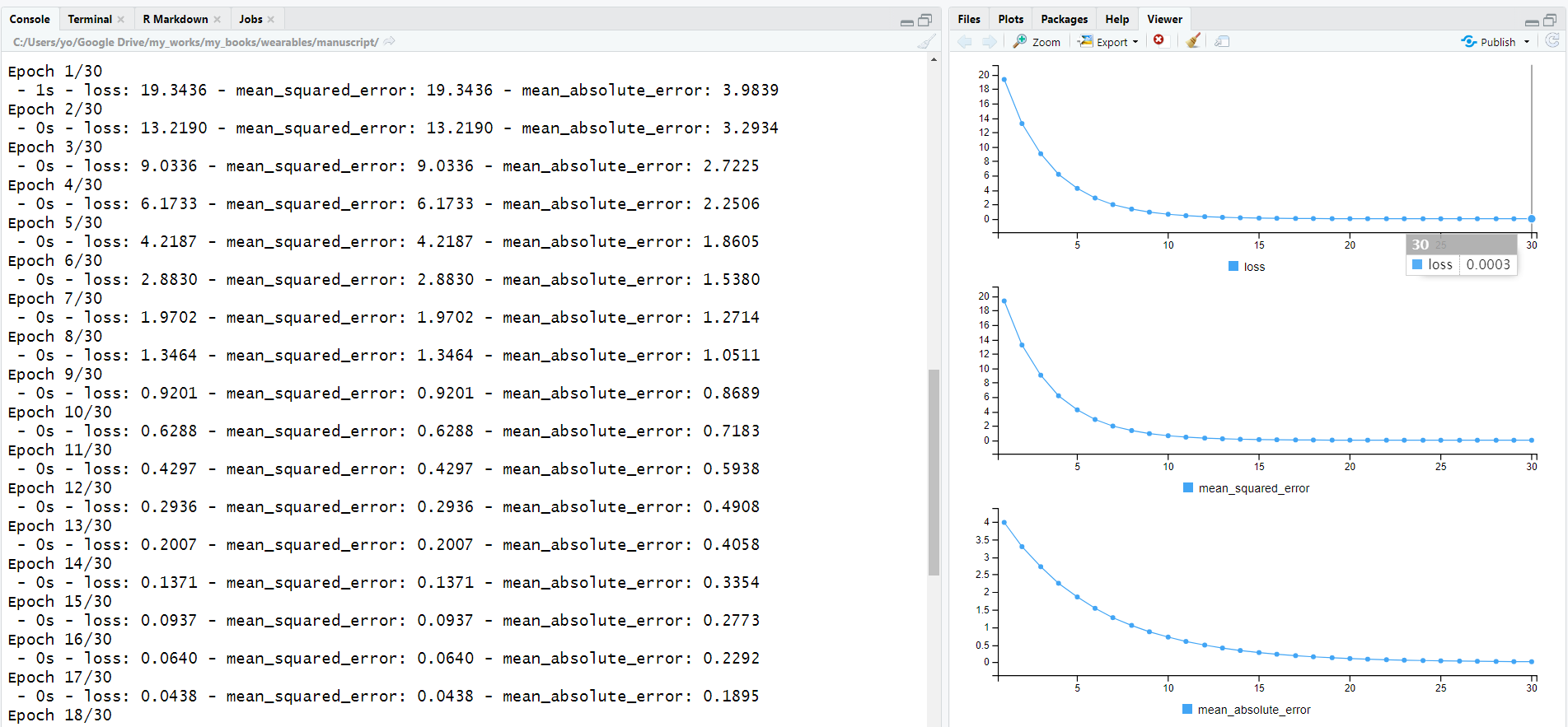
FIGURE 8.17: fit() function output.
The information saved in the history variable can be plotted with plot(history). This will generate plots for the loss, MSE, and MAE.
Once the model is trained, we can perform inference on new data points with the predict_on_batch() function. Here we are passing three data points.
model %>% predict_on_batch(c(7, 50, -220))
#>  [,1]
#>  [1,]    3.465378
#>  [2,]   24.752701
#>  [3,] -108.911880
Now, try setting a higher learning rate, for example, \(0.05\). With this learning rate, the algorithm will converge much faster. In my computer, at epoch \(11\) the loss was already \(0\).
compile() or fit() functions, you will have to rerun the code that instantiates and defines the network. This is because the model object saves the current state including the learned weights. If you rerun the fit() function on a previously trained model, it will start with the previously learned weights.
8.3 Classification with Neural Networks
Neural networks are trained iteratively by modifying their weights while aiming to minimize the loss function. When the network predicts real numbers, the MSE loss function is normally used. For classification problems, the network should predict the most likely class out of \(k\) possible categories. To make a neural network work for classification problems, we need to introduce new elements to its architecture:
- Add more units to the output layer.
- Use a softmax activation function in the output layer.
- Use average cross-entropy as the loss function.
Let’s start with point number \(1\) (add more units to the output layer). This means that if the number of classes is \(k\), then the last layer needs to have \(k\) units, one for each class. That’s it! Figure 8.18 shows an example of a neural network with an output layer having \(3\) units. Each unit predicts a score for each of the \(3\) classes. Let’s call the vector of predicted scores \(y'\).
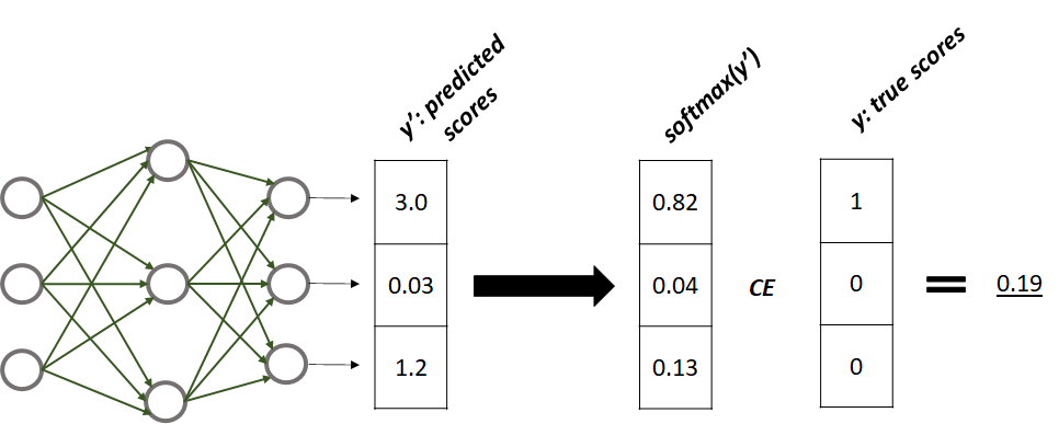
FIGURE 8.18: Neural network with 3 output scores. Softmax is applied to the scores and the cross-entropy with the true scores is calculated. This gives us an estimate of the similarity between the network’s predictions and the true values.
Point number \(2\) says that a softmax activation function should be used in the output layer. When training the network, just as with regression, we need a way to compute the error between the predicted values \(y'\) and the true values \(y\). In this case, \(y\) is a one-hot encoded vector with a \(1\) at the position of the true class and \(0s\) elsewhere. If you are not familiar with one-hot encoding, you can check the topic in chapter 5. As opposed to other classifiers like decision trees, \(k\)-NN, etc., neural networks need the classes to be one-hot encoded.
With regression problems, one way to compare the prediction with the true value is by using the squared difference: \((y' - y)^2\). With classification, \(y\) and \(y'\) are vectors so we need another way to compare them. The true values \(y\) are represented as a vector of probabilities with a \(1\) at the position of the true class. The output scores \(y'\) do not necessarily sum up to \(1\) thus, they are not proper probabilities. Before comparing \(y\) and \(y'\) we need both to be probabilities. The softmax activation function is used to convert \(y'\) into a vector of probabilities. The softmax function is applied individually to each element of a vector:
\[\begin{equation} softmax(\boldsymbol{x},i) = \frac{e^{\boldsymbol{x}_i}}{\sum_{j}{e^{\boldsymbol{x}_j}}} \tag{8.9} \end{equation}\]
where \(\boldsymbol{x}\) is a vector and \(i\) is an index pointing to a particular element in the vector. Thus, to convert \(y'\) into a vector of probabilities we need to apply softmax to each of its elements. One thing to note is that this activation function depends on all the values in the vector (the output values of all units). Figure 8.18 shows the resulting vector of probabilities after applying softmax to each element of \(y'\). In R this can be implemented like the following:
# Scores from the figure.
scores <- c(3.0, 0.03, 1.2)

# Softmax function.
softmax <- function(scores){
  exp(scores) / sum(exp(scores))
}
probabilities <- softmax(scores)
print(probabilities)
#> [1] 0.82196 0.04217 0.13587
print(sum(probabilities)) # Should sum up to 1.
#> [1] 1
We used R’s vectorization capabilities to compute the final vector of probabilities within the same function without having to iterate through each element. When using Keras, these operations are efficiently computed by the backend (for example, TensorFlow).
Finally, point \(3\) states that we need to use average cross-entropy as the loss function. Now that we have converted \(y'\) into probabilities, we can compute its dissimilarity with \(y\). The distance (dissimilarity) between two vectors (\(A\),\(B\)) of probabilities can be computed using cross-entropy:
\[\begin{equation} CE(A,B) = - \sum_{i}{B_i log(A_i)} \tag{8.10} \end{equation}\]
Thus, to get the dissimilarity between \(y'\) and \(y\) first we apply softmax to \(y'\) (to transform it into proper probabilities) and then, we compute the cross entropy between the resulting vector of probabilities and \(y\):
\[\begin{equation} CE(softmax(y'),y). \end{equation}\]
In R this can be implemented with the following:
# Cross-entropy
CE <- function(A,B){
 - sum(B * log(A))
}

y <- c(1, 0, 0)

print(CE(softmax(scores), y))
#> [1] 0.1961Now we know how to compute the cross-entropy for each training instance. The total loss function is then, the average cross-entropy across the training points. The next section shows how to build a neural network for classification using Keras.
8.3.1 Classification of Electromyography Signals
keras_electromyography.R
In this example, we will train a neural network with Keras to classify hand gestures based on muscle electrical activity. The ELECTROYMYOGRAPHY dataset will be used here. The electrical activity was recorded with an electromyography (EMG) sensor worn as an armband. The data were collected and made available by Yashuk (2019). The armband device has \(8\) sensors which are placed on the skin surface and measure electrical activity from the right forearm at a sampling rate of \(200\) Hz. A video of the device can be found here: https://youtu.be/OuwDHfY2Awg
The data contains \(4\) different gestures: 0-rock, 1-scissors, 2-paper, 3-OK, and has \(65\) columns. The last column is the class label from \(0\) to \(3\). The first \(64\) columns are electrical measurements. \(8\) consecutive readings for each of the \(8\) sensors. The objective is to use the first \(64\) variables to predict the class.
The script keras_electromyography.R has the full code. We start by splitting the dataset into train (\(60\%\)), validation (\(10\%\)) and test (\(30\%\)) sets. We will use the validation set to monitor the performance during each epoch. We also need to normalize the three sets but only learn the normalization parameters from the train set. The normalize() function included in the script will do the job.
One last thing we need to do is to format the data as matrices and one-hot encode the class. The following code defines a function that takes as input a data frame and the expected number of classes. It assumes that the first columns are the features and the last column contains the class. First, it converts the features into a matrix and stores them in x. Then, it converts the class into an array and one-hot encodes it using the to_categorical() function from Keras. The classes are stored in y and the function returns a list with the features and one-hot encoded classes. Then, we can call the function with the train, validation, and test sets.
# Define a function to format features and one-hot encode the class.
format.to.array <- function(data, numclasses = 4){
  x <- as.matrix(data[, 1:(ncol(data)-1)])
  y <- as.array(data[, ncol(data)])
  y <- to_categorical(y, num_classes = numclasses)
  l <- list(x=x, y=y)
  return(l)
}

# Format data
trainset <- format.to.array(trainset, numclasses = 4)
valset <- format.to.array(valset, numclasses = 4)
testset <- format.to.array(testset, numclasses = 4)
Let’s print the first one-hot encoded classes from the train set:
head(trainset$y)

#>        [,1] [,2] [,3] [,4]
#> [1,]    0    0    1    0
#> [2,]    0    0    1    0
#> [3,]    0    0    1    0
#> [4,]    0    0    0    1
#> [5,]    1    0    0    0
#> [6,]    0    0    0    1
The first three instances belong to the class ‘paper’ because the \(1s\) are in the third position. The corresponding integers are 0-rock, 1-scissors, 2-paper, 3-OK. So ‘paper’ comes in the third position. The fourth instance belongs to the class ‘OK’, the fifth to ‘rock’, and so on.
Now it’s time to define the neural network architecture! We will do so inside a function:
# Define the network's architecture.
get.nn <- function(ninputs = 64, nclasses = 4, lr = 0.01){

  model <- keras_model_sequential()

  model %>%
    layer_dense(units = 32, activation = 'relu',
                input_shape = ninputs) %>%
    layer_dense(units = 16, activation = 'relu') %>%
    layer_dense(units = nclasses, activation = 'softmax')

  model %>% compile(
    loss = 'categorical_crossentropy',
    optimizer = optimizer_sgd(lr = lr),
    metrics = c('accuracy')
  )

  return(model)
}
The first argument takes the number of inputs (features), the second argument specifies the number of classes and the last argument is the learning rate \(\alpha\). The first line instantiates an empty keras sequential model. Then we add three layers. The first two are hidden layers and the last one will be the output layer. The input layer is implicitly defined when setting the input_shape parameter in the first layer. The first hidden layer has \(32\) units with a ReLU activation function. Since this is the first hidden layer, we also need to specify what is the expected input by setting the input_shape. In this case, the number of input features is \(64\). The next hidden layer has \(16\) ReLU units. For the output layer, the number of units needs to be equal to the number of classes (\(4\), in this case). Since this is a classification problem we also set the activation function to softmax.
Then, the model is compiled and the loss function is set to categorical_crossentropy because this is a classification problem. Stochastic gradient descent is used with a learning rate passed as a parameter. During training, we want to monitor the accuracy. Finally, the function returns the compiled model.
Now we can call our function to create the model. This one will have \(64\) inputs and \(4\) outputs and the learning rate is set to \(0.01\). It is always useful to print a summary of the model with the summary() function.
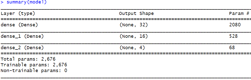
FIGURE 8.19: Summary of the network.
From the summary, we can see that the network has \(3\) layers. The second column shows the output shape which in this case corresponds to the number of units in each layer. The last column shows the number of parameters of each layer. For example, the first layer has \(2080\) parameters! Those come from the weights and biases. There are \(64\) (inputs) * \(32\) (units) = \(2048\) weights plus the \(32\) biases (one for each unit). The biases are included by default on each layer unless otherwise specified.
The second layer receives \(32\) inputs on each of its \(16\) units. Thus \(32\) * \(16\) + \(16\) (biases) = \(528\). The last layer has \(16\) inputs from the previous layer on each of its \(4\) units plus \(4\) biases giving a total of \(68\) parameters. In total, the network has \(2676\) parameters. Here, we see how fast the number of parameters grows when adding more layers and units. Now, we use the fit() function to train the model.
history <- model %>% fit(
  trainset$x, trainset$y,
  epochs = 300,
  batch_size = 8,
  validation_data = list(valset$x, valset$y),
  verbose = 1,
  view_metrics = TRUE
)
The model is trained for \(300\) epochs with a batch size of \(8\). We used the validation_data parameter to specify the validation set to compute the performance on unseen data. The training will take some minutes to complete. Bigger models can take hours or even several days. Thus, it is a good idea to save a model once it is trained. You can do so with the save_model_hdf5() or save_model_tf() methods. The former saves the model in hdf5 format while the later saves it in TensorFlow’s SavedModel format. The SavedModel is stored as a directory containing the necessary serialized files to restore the model’s state.
# Save model as hdf5.
save_model_hdf5(model, "electromyography.hdf5")

# Alternatively, save model as SavedModel.
save_model_tf(model, "electromyography_tf")
We can load a previously saved model with:
# Load model.
model <- load_model_hdf5("electromyography.hdf5")

# Or alternatively if the model is in SavedModel format.
model <- load_model_tf("electromyography")hdf5 and SavedModel versions are included.
hdf5 files. AttributeError: 'str' object has no attribute 'decode'. If you encounter this error, load the models in SavedModel format using the load_model_tf() method instead.
Figure 8.20 shows the train and validation loss and accuracy as produced by plot(history). We see that both the training and validation loss are decreasing over time. The accuracy increases over time.
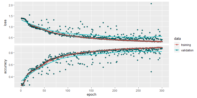
FIGURE 8.20: Loss and accuracy of the electromyography model.
Now, we evaluate the performance of the trained model with the test set using the evaluate() function.
The accuracy was pretty decent (\(\approx 84\%\)). To get the actual class predictions you can use the predict_classes() function.
Note that this function returns the classes with numbers starting with \(0\) just as in the original dataset.
Sometimes it is useful to access the actual predicted scores for each class. This can be done with the predict_on_batch() function.
# Make predictions on the test set.
predictions <- model %>% predict_on_batch(testset$x)
head(predictions)
#>              [,1]         [,2]         [,3]         [,4]
#> [1,] 1.957638e-05 8.726048e-02 7.708290e-01 1.418910e-01
#> [2,] 3.937355e-05 2.571992e-04 9.965665e-01 3.136863e-03
#> [3,] 4.261451e-03 7.343097e-01 7.226156e-02 1.891673e-01
#> [4,] 8.669784e-06 2.088269e-04 1.339851e-01 8.657974e-01
#> [5,] 9.999956e-01 7.354113e-26 1.299388e-08 4.451362e-06
#> [6,] 2.513005e-05 9.914154e-01 7.252949e-03 1.306421e-03
To obtain the actual classes from the scores, we can compute the index of the maximum column. Then we subtract \(-1\) so the classes start at \(0\).
Since the true classes are also one-hot encoded we need to do the same to get the ground truth.
groundTruth <- max.col(testset$y) - 1

# Compute accuracy.
sum(classes == groundTruth) / length(classes)
#> [1] 0.8474576
The integers are mapped to class strings. Then, a confusion matrix is generated.
# Convert classes to strings.
# Class mapping by index: rock 0, scissors 1, paper 2, ok 3.
mapping <- c("rock", "scissors", "paper", "ok")
# Need to add 1 because indices in R start at 1.
str.predictions <- mapping[classes+1]
str.groundTruth <- mapping[groundTruth+1]

library(caret)
cm <- confusionMatrix(as.factor(str.predictions),
                      as.factor(str.groundTruth))
cm$table
#>           Reference
#> Prediction  ok paper rock scissors
#>   ok       681   118   24       27
#>   paper     54   681   47       12
#>   rock      29    18  771        1
#>   scissors 134    68    8      867
Now, try to modify the network by making it deeper (adding more layers) and fine-tune the hyperparameters like the learning rate, batch size, etc., to increase the performance.
8.4 Overfitting
One important thing to look at when training a network is overfitting. That is, when the model memorizes instead of learning (see chapter 1). Overfitting means that the model becomes very specialized at mapping inputs to outputs from the train set but fails to do so with new test samples. One reason is that a model can become too complex and with so many parameters that it will perfectly adapt to its training data but will miss more general patterns preventing it to perform well on unseen instances. To diagnose this, one can plot loss/accuracy curves during training epochs.
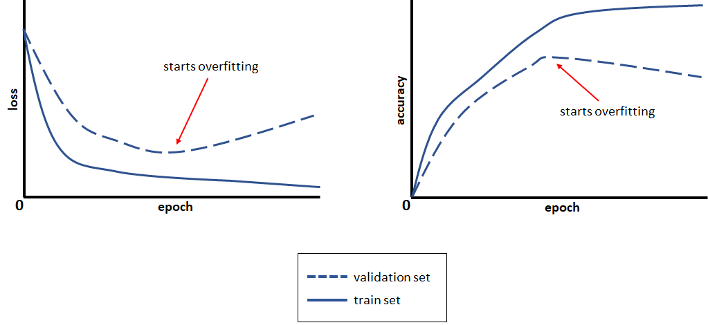
FIGURE 8.21: Loss and accuracy curves.
In Figure 8.21 we can see that after some epochs the validation loss starts to increase even though the train loss is still decreasing. This is because the model is getting better on reducing the error on the train set but its performance starts to decrease when presented with new instances. Conversely, one can observe a similar effect with the accuracy. The model keeps improving its performance on the train set but at some point, the accuracy on the validation set starts to decrease. Usually, one stops the training before overfitting starts to occur. In the following, I will introduce you to two common techniques to combat overfitting in neural networks.
8.4.1 Early Stopping
keras_electromyography_earlystopping.R
Neural networks are trained for several epochs using gradient descent. But the question is: For how many epochs?. As can be seen in Figure 8.21, too many epochs can lead to overfitting and too few can cause underfitting. Early stopping is a simple but effective method to reduce the risk of overfitting. The method consists of setting a large number of epochs and stop updating the network’s parameters when a condition is met. For example, one condition can be to stop when there is no performance improvement on the validation set after \(n\) epochs or when there is a decrease of some percent in accuracy.
Keras provides some mechanisms to implement early stopping and this is accomplished via callbacks. A callback is a function that is run at different stages during training such as at the beginning or end of an epoch or at the beginning or end of a batch operation. Callbacks are passed as a list to the fit() function. You can define custom callbacks or use some of the built-in ones including callback_early_stopping(). This callback will cause the training to stop when a metric stops improving. The metric can be accuracy, loss, etc. The following callback will stop the training if after \(10\) epochs (patience) there is no improvement of at least \(1\%\) (min_delta) in accuracy on the validation set.
callback_early_stopping(monitor = "val_acc",
                        min_delta = 0.01,
                        patience = 10,
                        verbose = 1,
                        mode = "max")
The min_delta parameter specifies the minimum change in the monitored metric to qualify as an improvement. The mode specifies if training should be stopped when the metric has stopped decreasing, if it is set to "min". If it is set to "max", training will stop when the monitored metric has stopped increasing.
It may be the case that the best validation performance was achieved not in the last epoch but at some previous point. By setting the restore_best_weights parameter to TRUE the model weights from the epoch with the best value of the monitored metric will be restored.
The script keras_electromyography_earlystopping.R shows how to use the early stopping callback in Keras with the electromyography dataset. The following code is an extract that shows how to define the callback and pass it to the fit() function.
# Define early stopping callback.
my_callback <- callback_early_stopping(monitor = "val_acc",
                                            min_delta = 0.01,
                                            patience = 50,
                                            verbose = 1,
                                            mode = "max",
                                            restore_best_weights = TRUE)

history <- model %>% fit(
  trainset$x, trainset$y,
  epochs = 500,
  batch_size = 8,
  validation_data = list(valset$x, valset$y),
  verbose = 1,
  view_metrics = TRUE,
  callbacks = list(my_callback)
)
This code will cause the training to stop if after \(50\) epochs there is no improvement in accuracy of at least \(1\%\) and will restore the model’s weights to the ones during the epoch with the highest accuracy. Figure 8.22 shows how the training stopped at epoch \(241\).
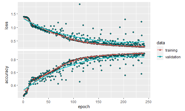
FIGURE 8.22: Early stopping example.
If we evaluate the final model on the test set, we see that the accuracy is \(86.4\%\), a noticeable increase compared to the \(84.7\%\) that we got when training for \(300\) epochs without early stopping.
8.4.2 Dropout
Dropout is another technique to reduce overfitting proposed by Srivastava et al. (2014). It consists of ‘dropping’ some of the units from a hidden layer for each sample during training. In theory, it can also be applied to input and output layers but that is not very common. The incoming and outgoing connections of a dropped unit are discarded. Figure 8.23 shows an example of applying dropout to a network. In Figure 8.23 b, the middle unit was removed from the network whereas in Figure 8.23 c, the top and bottom units were removed.
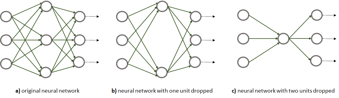
FIGURE 8.23: Dropout example.
Each unit has an associated probability \(p\) (independent of other units) of being dropped. This probability is another hyperparameter but typically it is set to \(0.5\). Thus, during each iteration and for each sample, half of the units are discarded. The effect of this, is having more simple networks (see Figure 8.23) and thus, less prone to overfitting. Intuitively, you can also think of dropout as training an ensemble of neural networks, each having a slightly different structure.
From the perspective of one unit that receives inputs from the previous hidden layer with dropout, approximately half of its incoming connections will be gone (if \(p=0.5\)). See Figure 8.24.
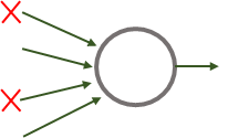
FIGURE 8.24: Incoming connections to one unit when the previous layer has dropout.
Dropout has the effect of making units not to rely on any single incoming connection. This makes the whole network able to compensate for the lack of connections by learning alternative paths. In practice and for many applications, this results in a more robust model. A side effect of applying dropout is that the expected value of the activation function of a unit will be diminished because some of the previous activations will be \(0\). Recall that the output of a neuron is computed as:
\[\begin{equation} f(\boldsymbol{x}) = g(\boldsymbol{w} \cdot \boldsymbol{x} + b) \end{equation}\]
where \(\boldsymbol{x}\) contains the input values from the previous layer, \(\boldsymbol{w}\) the corresponding weights and \(g()\) is the activation function. With dropout, approximately half of the values of \(\boldsymbol{x}\) will be \(0\) (if \(p=0.5\)). To compensate for that, the input values need to be scaled, in this case, by a factor of \(2\).
\[\begin{equation} f(\boldsymbol{x}) = g(\boldsymbol{w} \cdot 2 \boldsymbol{x} + b) \end{equation}\]
In modern implementations, this scaling is done during training so at inference time
there is no need to apply dropout. The predictions are done as usual. In Keras, the layer_dropout() can be used to add dropout to any layer. Its parameter rate is a float between \(0\) and \(1\) that specifies the fraction of units to drop. The following code snippet builds a neural network with \(2\) hidden layers. Then, dropout with a rate of \(0.5\) is applied to both of them.
model <- keras_model_sequential()

  model %>%
    layer_dense(units = 256, activation = 'relu', input_shape = 1000) %>%
    layer_dropout(0.5) %>%
    layer_dense(units = 128, activation = 'relu') %>%
    layer_dropout(0.5) %>%
    layer_dense(units = 2, activation = 'softmax')
It is very common to apply dropout to networks in computer vision because the inputs are images or videos containing a lot of input values (pixels) but the number of samples is often very limited causing overfitting. In section 8.6 Convolutional Neural Networks (CNNs) will be introduced. They are suitable for computer vision problems. In the corresponding smile detection example (section 8.8), we will use dropout. When building CNNs, dropout is almost always added to the different layers.
8.5 Fine-tuning a Neural Network
When deciding for a neural network’s architecture, no formula will tell you how many hidden layers or number of units each layer should have. There is also no formula for determining the batch size, the learning rate, type of activation function, for how many epochs should we train the network, and so on. All those are called the hyperparameters of the network. Hyperparameter tuning is a complex optimization problem and there is a lot of research going on that tackles the issue from different angles. My suggestion is to start with a simple architecture that has been used before to solve a similar problem and then fine-tune it for your specific task. If you are not aware of such a network, there are some guidelines (described below) to get you started. Always keep in mind that those are only recommendations, so you do not need to abide by them and you should feel free to try configurations that deviate from those guidelines depending on your problem at hand.
Training neural networks is a time-consuming process, especially in deep networks. Training a network can take from several minutes to weeks. In many cases, performing cross-validation is not feasible. A common practice is to divide the data into train/validation/test sets. The training data is used to train a network with a given architecture and a set of hyperparameters. The validation set is used to evaluate the generalization performance of the network. Then, you can try different architectures and hyperparameters and evaluate the performance again and again with the validation set. Typically, the network’s performance is monitored during training epochs by plotting the loss and accuracy of the train and validation sets. Once you are happy with your model, you test its performance on the test set only once and that is the result that is reported.
Here are some starting point guidelines, however, also take into consideration that those hyperparameters can be dependent on each other. So, if you modify a hyperparameter it may impact other(s).
Number of hidden layers. Most of the time one or two hidden layers are enough to solve not too complex problems. One advice is to start with one hidden layer and if that one is not enough to capture the complexity of the problem, add another layer and so on.
Number of units. If a network has too few units it can underfit, that is, the model will be too simple to capture the underlying data patterns. If the network has too many units this can result in overfitting. Also, it will take more time to learn the parameters. Some guidelines mention that the number of units should be somewhere between the number of input features and the number of units in the output layer25. Guang-Bin Huang (2003) has even proposed a formula for the two-hidden layer case to calculate the number of units that are enough to learn \(N\) samples: \(2\sqrt{(m+2)N}\) where \(m\) is the number of output units.
My suggestion is to first gain some practice and intuition with simple problems. A good way to do so is with the TensorFlow playground (https://playground.tensorflow.org/) created by Daniel Smilkov and Shan Carter. This is a web-based implementation of a neural network that you can fine-tune to solve a predefined set of classification and regression problems. For example, Figure 8.25 shows how I tried to solve the XOR problem with a neural network with \(1\) hidden layer and \(1\) unit with a sigmoid activation function. After more than \(1,000\) epochs the loss is still quite high (\(0.38\)). Try to add more neurons and/or hidden layers and see if you can solve the XOR problem with fewer epochs.
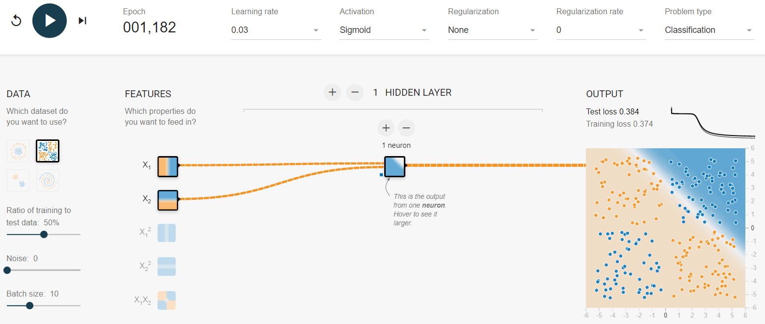
FIGURE 8.25: Screenshot of the TensorFlow playground. (Daniel Smilkov and Shan Carter, https://github.com/tensorflow/playground (Apache License 2.0)).
Batch size. Batch sizes typically range between \(4\) and \(512\). Big batch sizes provide a better estimate of the gradient but are more computationally expensive. On the other hand, small batch sizes are faster to compute but will incur in more noise in the gradient estimation requiring more epochs to converge. When using a GPU or other specialized hardware, the computations can be performed in parallel thus, allowing bigger batch sizes to be computed in a reasonable time. Some people argue that the noise introduced with small batch sizes is good to escape from local minima. Keskar et al. (2016) showed that in practice, big batch sizes can result in degraded models. A good starting point is \(32\) which is the default in Keras.
Learning rate. This is one of the most important hyperparameters. The learning rate specifies how fast gradient descent ‘moves’ when trying to find an optimal minimum. However, this doesn’t mean that the algorithm will learn faster if the learning rate is set to a high value. If it is too high, the loss can start oscillating. If it is too low, the learning will take a lot of time. One way to fine-tune it, is to start with the default one. In Keras, the default learning rate for stochastic gradient descent is \(0.01\). Then, based on the loss plot across epochs, you can decrease/increase it. If learning is taking long, try to increase it. If the loss seems to be oscillating or stuck, try reducing it. Typical values are \(0.1\), \(0.01\), \(0.001\), \(0.0001\), \(0.00001\). Additionally to stochastic gradient descent, Keras provides implementations of other optimizers26 like Adam27 which have adaptive learning rates, but still, one needs to specify an initial one.
8.6 Convolutional Neural Networks
Convolutional Neural Networks or CNNs for short, have become extremely popular due to their capacity to solve computer vision problems. Most of the time they are used for image classification tasks but can also be used for regression and for time series data. If we wanted to perform image classification with a traditional neural network, first we would need to either build a feature vector by:
- extracting features from the image or,
- flattening the image pixels into a 1D array.
The first solution requires a lot of image processing expertise and domain knowledge. Extracting features from images is not a trivial task and requires a lot of preprocessing to reduce noise, artifacts, segment the objects of interest, remove background, etc. Additionally, considerable effort is spent on feature engineering. The drawback of the second solution is that spatial information is lost, that is, the relationship between neighboring pixels. CNNs solve the two previous problems by automatically extracting features while preserving spatial information. As opposed to traditional networks, CNNs can take as input \(n\)-dimensional images and process them efficiently. The main building blocks of a CNN are:
- Convolution layers
- Pooling operations
- Traditional fully connected layers
Figure 8.26 shows a simple CNN and its basic components. First, the input image goes through a convolution layer with \(4\) kernels (details about the convolution operation are described in the next subsection). This layer is in charge of extracting features by applying the kernels on top of the image. The result of this operation is a convolved image, also known as feature maps. The number of feature maps is equal to the number of kernels, in this case, \(4\). Then, a pooling operation is applied on top of the feature maps. This operation reduces the size of the feature maps by downsampling them (details on this in a following subsection). The output of the pooling operation is a set of feature maps with reduced size. Here, the outputs are \(4\) reduced feature maps since the pooling operation is applied to each feature map independently of the others. Then, the feature maps are flattened into a one-dimensional array. Conceptually, this array represents all the features extracted from the previous steps. These features are then used as inputs to a neural network with its respective input, hidden, and output layers. An ’*’ and underlined text means that parameter learning occurs in that layer. For example, in the convolution layer, the parameters of the kernels need to be learned. On the other hand, the pooling operation does not require parameter learning since it is a fixed operation. Finally, the parameters of the neural network are learned too, including the hidden layers and the output layer.
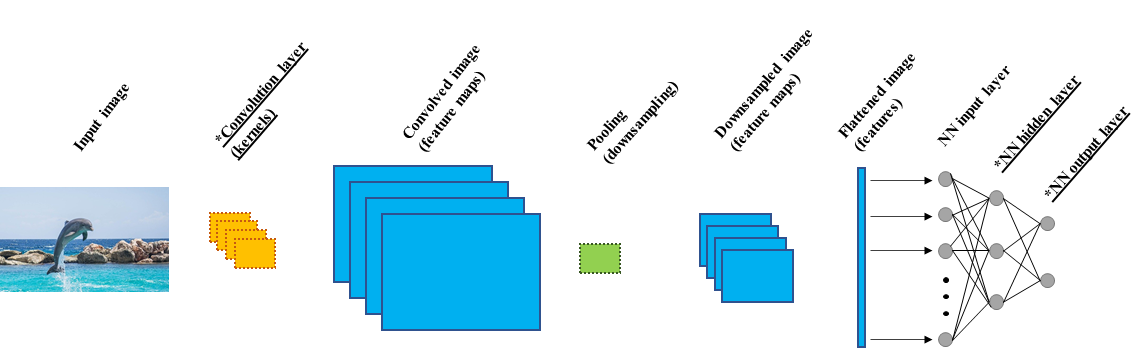
FIGURE 8.26: Simple CNN architecture. An `*’ indicates that parameter learning occurs.
One can build more complex CNNs by stacking more convolution layers and pooling operations. By doing so, the level of abstraction increases. For example, the first convolution extracts simple features like horizontal, vertical, diagonal lines, etc. The next convolution could extract more complex features like squares, triangles, and so on. The parameter learning of all layers (including the convolution layers) occurs during the same forward and backpropagation step just as with a normal neural network. Both, the features and the classification task are learned at the same time! During learning, batches of images are forward propagated and the parameters are adjusted accordingly to minimize the error (for example, the average cross-entropy for classification). The same methods for training normal neural networks are used for CNNs, for example, stochastic gradient descent.
At inference time, the convolution layers and pooling operations act as feature extractors by generating feature maps that are ultimately flattened and passed to a normal neural network. It is also common to use the first layers as feature extractors and then replace the neural network with another model (Random Forest, SVM, etc.). In the following sections, details about the convolution and pooling operations are presented.
8.6.1 Convolutions
Convolutions are used to automatically extract feature maps from images. A convolution operation consists of a kernel also known as a filter which is a matrix with real values. Kernels are usually much smaller than the original image. For example, for a grayscale image of height and width of \(100\)x\(100\) a typical kernel size would be \(3\)x\(3\). The size of the kernel is a hyperparameter. The convolution operation consists of applying the kernel over the image starting at the upper left corner and moving forward row by row until reaching the bottom right corner. The stride controls how many elements the kernel is moved at a time and this is also a hyperparameter. A typical value for the stride is \(1\).
The convolution operation computes the sum of the element-wise product between the kernel and the image region it is covering. The output of this operation is used to generate the convolved image (feature map). Figure 8.27 shows the first two iterations and the final iteration of the convolution operation on an image. In this case, the kernel is a \(3\)x\(3\) matrix with \(1\)s in its first row and \(0\)s elsewhere. The original image has a size of \(5\)x\(5\)x\(1\) (height, width, depth) and it seems to be a number \(7\).
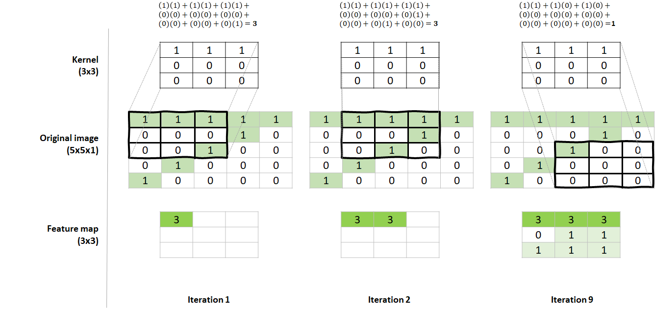
FIGURE 8.27: Convolution operation with a kernel of size 3x3 and stride=1. Iterations 1, 2, and 9.
In the first iteration, the kernel is aligned with the upper left corner of the original image. An element-wise multiplication is performed and the results are summed. The operation is shown at the top of the figure. In the first iteration, the result was \(3\) and it is set at the corresponding position of the final convolved image (feature map). In the next iteration, the kernel is moved one position to the right and again, the final result is \(3\) which is set in the next position of the convolved image. The process continues until the kernel reaches the bottom right corner. At the last iteration (9), the result is \(1\).
Now, the convolved image (feature map) represents the features extracted by this particular kernel. Also, note that the feature map is a \(3\)x\(3\) matrix which is smaller than the original image. It is also possible to force the feature map to have the same size as the original image by padding it with zeros.
Before learning starts, the kernel values are initialized at random. In this example, the kernel has \(1\)s in the first row and it has \(3\)x\(3=9\) parameters. This is what makes CNNs so efficient since the same kernel is applied to the entire image. This is known as ‘parameter sharing’. Our kernel has \(1\)s at the top and \(0\)s elsewhere so it seems that this kernel learned to detect horizontal lines. If we look at the final convolved image, we see that the horizontal lines were emphasized by this kernel. This would be a good candidate kernel to differentiate between \(7\)s and \(0\)s, for example. Since \(0\)s does not have long horizontal lines. But maybe it will have difficulties discriminating between \(7\)s and \(5\)s since both have horizontal lines at the top.
In this example, only \(1\) kernel was used but in practice, you may want more kernels, each in charge of identifying the best features for the given problem. For example, another kernel could learn to identify diagonal lines which would be useful to differentiate between \(7\)s and \(5\)s. The number of kernels per convolution layer is a hyperparameter. In the previous example, we could have defined to have \(4\) kernels instead of one. In that case, the output of that layer would have been \(4\) feature maps of size \(3\)x\(3\) each (Figure 8.28).
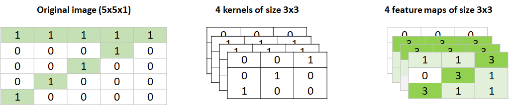
FIGURE 8.28: A convolution with 4 kernels. The output is 4 feature maps.
What would be the output of a convolution layer with \(4\) kernels of size \(3\)x\(3\) if it is applied to an RGB color image of size \(5\)x\(5\)x\(3\))? In that case, the output will be the same (\(4\) feature maps of size \(3\)x\(3\)) as if the image were in grayscale (\(5\)x\(5\)x\(1\)). Remember that the number of output feature maps is equal to the number of kernels regardless of the depth of the image. However, in this case, each kernel will have a depth of \(3\). Each depth is applied independently to the corresponding R, G, and B image channels. Thus, each kernel has \(3\)x\(3\)x\(3=27\) parameters that need to be learned. After applying each kernel to each image channel (in this example, \(3\) channels), the results of each channel are added and this is why we end up with one feature map per kernel. The following course website has a nice interactive animation of how convolutions are applied to an image with \(3\) channels: https://cs231n.github.io/convolutional-networks/. In the next section (‘CNNs with Keras’), a couple of examples that demonstrate how to calculate the number of parameters and the outputs’ shape will be presented as well.
8.6.2 Pooling Operations
Pooling operations are typically applied after convolution layers. Their purpose is to reduce the size of the data and to emphasize important regions. These operations perform a fixed computation on the image and do no have learnable parameters. Similar to kernels, we need to define a window size. Then, this window is moved throughout the image and a computation is performed on the pixels covered by the window. The difference with kernels is that this window is just a guide but does not have parameters to be learned. The most common pooling operation is max pooling which consists of selecting the highest value. Figure 8.29 shows an example of a max pooling operation on a \(4\)x\(4\) image. The window size is \(2\)x\(2\) and the stride is \(2\). The latter means that the window moves \(2\) places at a time.
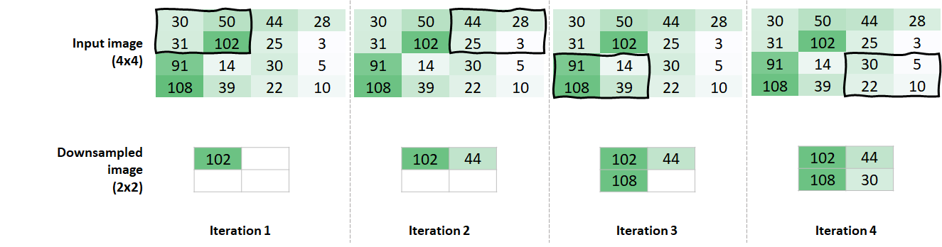
FIGURE 8.29: Max pooling with a window of size 2x2 and stride = 2.
The result of this operation is an image of size \(2\)x\(2\) which is half of the original one. Aside from max pooling, average pooling can be applied instead. In that case, it computes the mean value across all values covered by the window.
8.7 CNNs with Keras
Keras provides several functions to define convolution layers and pooling operations. In TensorFlow, image dimensions are specified with the following order: height, width, and depth. In Keras, the layer_conv_2d() function is used to add a convolution layer to a sequential model. This function has several arguments but the \(6\) most common ones are: filters,kernel_size,strides,padding,activation, and input_shape.
# Convolution layer.
layer_conv_2d(filters = 4, # Number of kernels.
                kernel_size = c(3,3), # Kernel size.
                strides = c(1,1), # Stride.
                padding = "same", # Type of padding.
                activation = 'relu', # Activation function.
                input_shape = c(5,5,1)) # Input image dimensions.
                                        # Only specified in first layer.
The filters parameter specifies the number of kernels. The kernel_size specifies the kernel size (height, width). The strides is an integer or list of \(2\) integers, specifying the strides of the convolution along the width and height (the default is \(1\)). The padding can take two possible strings: "same" or "valid". If padding="same" the input image will be padded with zeros based on the kernel size and strides such that the convolved image has the same size as the original one. If padding="valid" it means no padding is applied. The default is "valid". The activation parameter takes as input a string with the name of the activation function to use. The input_shape parameter is required when this layer is the first one and specifies the dimensions of the input image.
To add a max pooling operation you can use the layer_max_pooling_2d() function. Its most important parameter is pool_size.
The pool_size specifies the window size (height, width). By default, the strides will be equal to pool_size but if desired, this can be changed with the strides parameter. This function also accepts a padding parameter similar to the one for layer_max_pooling_2d().
pool_size parameter).
To illustrate this convolution and pooling operations I will use two simple examples. The complete code for the two examples can be found in the script keras_cnns.R.
8.7.1 Example 1
Let’s create our first CNN in Keras. For now, this CNN will not be trained but only its architecture will be defined. The objective is to understand the building blocks of the network. In the next section, we will build and train a CNN that detects smiles from image faces.
Our network will consist of \(1\) convolution layer, \(1\) max pooling layer, \(1\) fully connected hidden layer, and \(1\) output layer as if this were a classification problem. The code to build such a network is shown below and the output of the summary() function in Figure 8.30.
library(keras)

model <- keras_model_sequential()

model %>%
  layer_conv_2d(filters = 4,
                kernel_size = c(3,3),
                padding = "valid",
                activation = 'relu',
                input_shape = c(10,10,1)) %>%
  layer_max_pooling_2d(pool_size = c(2, 2)) %>%
  layer_flatten() %>%
  layer_dense(units = 32, activation = 'relu') %>%
  layer_dense(units = 2, activation = 'softmax')

summary(model)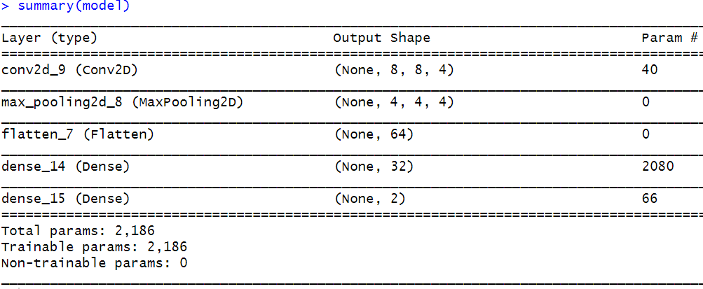
FIGURE 8.30: Output of summary().
The first convolution layer has \(4\) kernels of size \(3\)x\(3\) and a ReLU as the activation function. The padding is set to "valid" so no padding will be performed. The input image is of size \(10\)x\(10\)x\(1\) (height, width, depth). Then, we apply max pooling with a window size of \(2\)x\(2\). Later, the output is flattened and fed into a fully connected layer with \(32\) units. Finally, the output layer has \(2\) units with a softmax activation function for classification.
From the summary, the output of the first Conv2D layer is (None, 8, 8, 4). The ‘None’ means that the number of input images is not fixed and depends on the batch size. The next two numbers correspond to the height and width which are both \(8\). This is because the image was not padded and after applying the convolution operation on the original \(10\)x\(10\) height and width image, its dimensions are reduced to \(8\). The last number (\(4\)) is the number of feature maps which is equal to the number of kernels (filters=4). The number of parameters is \(40\) (last column). This is because there are \(4\) kernels with \(3\)x\(3=9\) parameters each, and there is one bias per kernel included by default: \(4 \times 3 \times 3 \times + 4 = 40\).
The output of MaxPooling2D is (None, 4, 4, 4). The height and width are \(4\) because the pool size was \(2\) and the stride was \(2\). This had the effect of reducing to half the height and width of the output of the previous layer. Max pooling preserves the number of feature maps, thus, the last number is \(4\) (the number of feature maps from the previous layer). Max pooling does not have any learnable parameters since it applies a fixed operation every time.
Before passing the downsampled feature maps to the next fully connected layer they need to be flattened into a \(1\)-dimensional array. This is done with the layer_flatten() function. Its output has a shape of (None, 64) which corresponds to the \(4 \times 4 \times 4 =64\) features of the previous layer. The next fully connected layer has \(32\) units each with a connection with every one of the \(64\) input features. Each unit has a bias. Thus the number of parameters is \(64 \times 32 + 32 = 2080\).
Finally the output layer has \(32 \times 2 + 2=66\) parameters. And the entire network has \(2,186\) parameters! Now, you can try to modify, the kernel size, the strides, the padding, and input shape and see how the output dimensions and the number of parameters vary.
8.7.2 Example 2
Now let’s try another example, but this time the input image will have a depth of \(3\) simulating an RGB image.
model2 <- keras_model_sequential()

model2 %>%
  layer_conv_2d(filters = 16,
                kernel_size = c(3,3),
                padding = "same",
                activation = 'relu',
                input_shape = c(28,28,3)) %>%
  layer_max_pooling_2d(pool_size = c(2, 2)) %>%
  layer_flatten() %>%
  layer_dense(units = 64, activation = 'relu') %>%
  layer_dense(units = 5, activation = 'softmax')

summary(model2)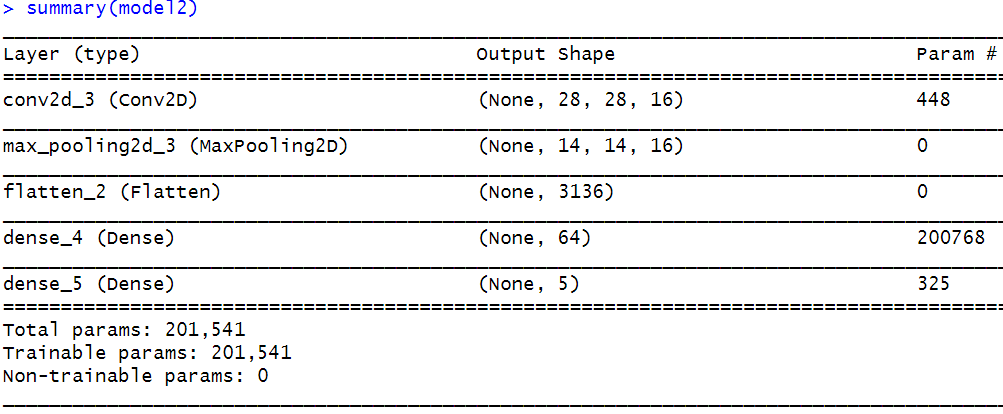
FIGURE 8.31: Output of summary().
Figure 8.31 shows that the output height and width of the first Conv2D layer is \(28\) which is the same as the input image size. This is because this time we set padding = "same" and the image dimensions were preserved. The \(16\) corresponds to the number of feature maps which was set with filters = 16.
The total parameter count for this layer is \(448\). Each kernel has \(3 \times 3 = 9\) parameters. There are \(16\) kernels but each kernel has a \(depth=3\) because the input image is RGB. \(9 \times 16[kernels] \times 3[depth] + 16[biases] = 448\). Notice that even though each kernel has a depth of \(3\) the output number of feature maps of this layer is \(16\) and not \(16 \times 3 = 48\). This is because as mentioned before, each kernel produces a single feature map regardless of the depth because the values are summed depth-wise. The rest of the layers are similar to the previous example.
8.8 Smiles Detection with a CNN
In this section, we will build a CNN that detects smiling and non-smiling faces from pictures from the SMILES dataset. This information could be used, for example, to analyze smiling patterns during job interviews, exams, etc. For this task, we will use a cropped (Sanderson and Lovell 2009) version of the Labeled Faces in the Wild (LFW) database (Gary B. Huang et al. 2008). A subset of the database was labeled by O. A. Arigbabu et al. (2016), O. Arigbabu (2017). The labels are provided as two text files, each, containing the list of files that correspond to smiling and non-smiling faces. The dataset can be downloaded from: http://conradsanderson.id.au/lfwcrop/ and the labels list from: https://data.mendeley.com/datasets/yz4v8tb3tp/5. See Appendix B for instructions on how to setup the dataset.
The smiling set has \(600\) pictures and the non-smiling has \(603\) pictures. Figure 8.32 shows an example of one image from each of the sets.
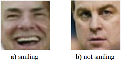
FIGURE 8.32: Example of a smiling and a non-smiling face. (Adapted from the LFWcrop Face Dataset: C. Sanderson, B.C. Lovell. “Multi-Region Probabilistic Histograms for Robust and Scalable Identity Inference.” Lecture Notes in Computer Science (LNCS), Vol. 5558, pp. 199-208, 2009. doi: https://doi.org/10.1007/978-3-642-01793-3_21).
The script keras_smile_detection.R has the full code of the analysis. First, we load the list of smiling pictures.
datapath <- file.path(datasets_path,"smiles")
smile.list <- read.table(paste0(datapath,"SMILE_list.txt"))
head(smile.list)
#> V1
#> 1     James_Jones_0001.jpg
#> 2     James_Kelly_0009.jpg
#> 3 James_McPherson_0001.jpg
#> 4      James_Watt_0001.jpg
#> 5     Jamie_Carey_0001.jpg
#> 6      Jamie_King_0001.jpg

# Substitute jpg with ppm.
smile.list <- gsub("jpg", "ppm", smile.list$V1)
The SMILE_list.txt points to the names of the pictures in jpg format, but they are actually stored as ppm files. Thus, the jpg extension is replaced by ppm with the gsub() function. Since the images are in ppm format, we can use the pixmap library (Bivand, Leisch, and Maechler 2011) to read and plot them. The print() function can be used to display the image properties. Here, we see that these are RGB images of \(64\)x\(64\) pixels.
library(pixmap)

# Read an smiling face.
img <- read.pnm(paste0(datapath,"faces/", smile.list[10]), cellres = 1)

# Plot the image.
plot(img)

# Print its properties.
print(img)

#> Pixmap image
#> Type          : pixmapRGB
#> Size          : 64x64
#> Resolution    : 1x1
#> Bounding box  : 0 0 64 64
Then, we load the images into two arrays smiling.images and nonsmiling.images (code omitted here). If we print the array dimensions we see that there are \(600\) smiling images of size \(64 \times 64 \times 3\).
If we print the minimum and maximum values we see that they are \(0\) and \(1\) so there is no need for normalization.
The next step is to randomly split the dataset into train and test sets. We will use \(85\%\) for the train set and \(15\%\) for the test set. We set the validation_split parameter of the fit() function to choose a small percent (\(10\%\)) of the train set as the validation set during training.
After creating the train and test sets, the train set images and labels are stored in trainX and trainY, respectively and the test set data is stored in testX and testY. The labels in trainY and testY were one-hot encoded. Now that the data is in place, let’s build the CNN.
model <- keras_model_sequential()

model %>%
  layer_conv_2d(filters = 8,
                kernel_size = c(3,3),
                activation = 'relu',
                input_shape = c(64,64,3)) %>%
  layer_max_pooling_2d(pool_size = c(2, 2)) %>%
  layer_dropout(0.25) %>%
  layer_conv_2d(filters = 16,
                kernel_size = c(3,3),
                activation = 'relu') %>%
  layer_max_pooling_2d(pool_size = c(2, 2)) %>%
  layer_dropout(0.25) %>%
  layer_flatten() %>%
  layer_dense(units = 32, activation = 'relu') %>%
  layer_dropout(0.5) %>%
  layer_dense(units = 2, activation = 'softmax')
Our CNN consists of two convolution layers each followed by a max pooling operation and dropout. The feature maps are then flattened and passed to a fully connected layer with \(32\) units followed by a dropout. Since this is a binary classification problem (‘smile’ vs. ‘non-smile’) the output layer has \(2\) units with a softmax activation function. Now the model can be compiled and the fit() function used to begin the training!
# Compile model.
model %>% compile(
  loss = 'categorical_crossentropy',
  optimizer = optimizer_sgd(lr = 0.01),
  metrics = c("accuracy")
)

# Fit model.
history <- model %>% fit(
  trainX, trainY,
  epochs = 50,
  batch_size = 8,
  validation_split = 0.10,
  verbose = 1,
  view_metrics = TRUE
)
We are using a stochastic gradient descent optimizer with a learning rate of \(0.01\) and cross-entropy as the loss function. We can use \(10\%\) of the train set as the validation set by setting validation_split = 0.10. Once the training is done, we can plot the loss and accuracy of each epoch.
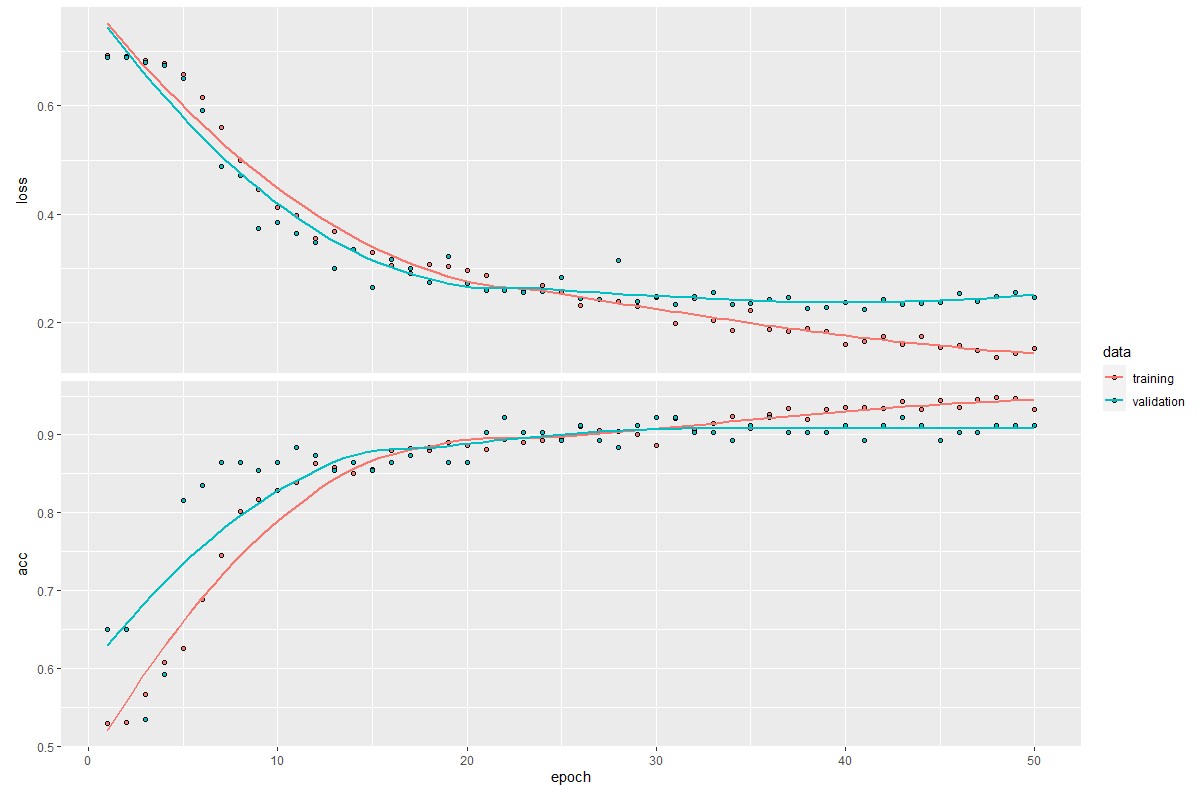
FIGURE 8.33: Train/test loss and accuracy.
After epoch \(25\) (see Figure 8.33) it looks like the training loss is decreasing faster than the validation loss. After epoch \(40\) it seems that the model starts to overfit (the validation loss is increasing a bit). If we look at the validation accuracy, it seems that it starts to get flat after epoch \(30\). Now we evaluate the model on the test set:
# Evaluate model on test set.
model %>% evaluate(testX, testY)
#> $loss
#> [1] 0.1862139

#> $acc
#> [1] 0.9222222
An accuracy of \(92\%\) is pretty decent if we take into account that we didn’t have to do any image preprocessing or feature extraction! We can print the predictions of the first \(16\) test images (see Figure 8.34).
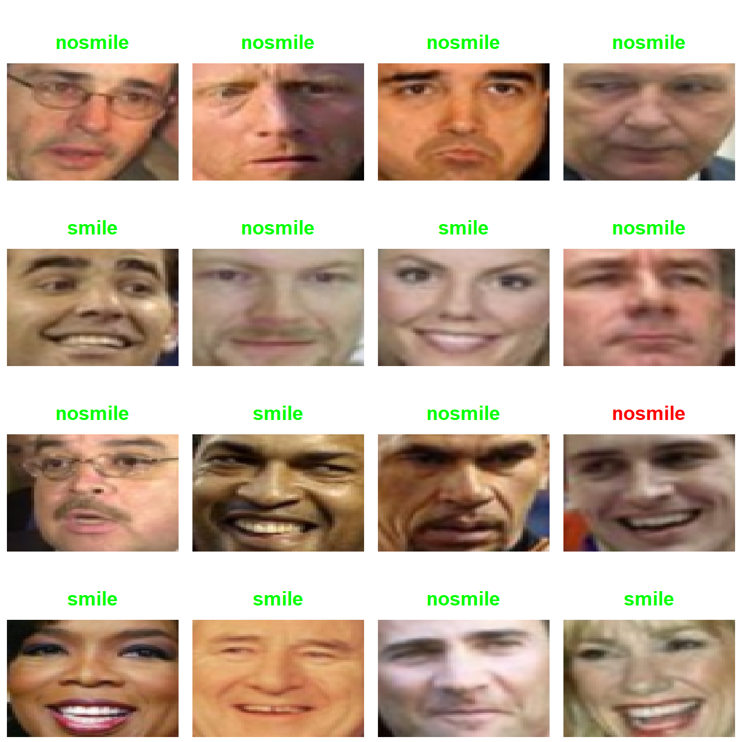
FIGURE 8.34: Predictions of the first \(16\) test set images. Correct predictions are in green and incorrect ones in red. (Adapted from the LFWcrop Face Dataset: C. Sanderson, B.C. Lovell. “Multi-Region Probabilistic Histograms for Robust and Scalable Identity Inference.” Lecture Notes in Computer Science (LNCS), Vol. 5558, pp. 199-208, 2009. doi: https://doi.org/10.1007/978-3-642-01793-3_21).
From those \(16\), all but one were correctly classified. The correct ones are shown in green and the incorrect one in red. Some faces seem to be smiling (last row, third image) but the mouth is closed, though. It seems that this CNN classifies images as ‘smiling’ only when the mouth is open which may be the way the train labels were defined.
8.9 Summary
Deep learning (DL) consists of a set of different architectures and algorithms. As of now, it mainly focuses on artificial neural networks (ANNs). This chapter introduced two main types of DL models (ANNs and CNNs) and their application to behavior analysis.
- Artificial neural networks (ANNs) are mathematical models inspired by the brain. But that does not mean they work the same as the brain.
- The perceptron is one of the simplest ANNs.
- ANNs consist of an input layer, hidden layer(s) and an output layer.
- Deep networks have many hidden layers.
- Gradient descent can be used to learn the parameters of a network.
- Overfitting is a recurring problem in ANNs. Some methods like dropout and early stopping can be used to reduce the effect of overfitting.
- A Convolutional Neural Network (CNN) is a type of ANN that can process \(N\)-dimensional arrays very efficiently. They are used mainly for computer vision tasks.
- CNNs consist of convolution and pooling layers.