Chapter 2 Predicting Behavior with Classification Models

In the previous chapter, the concept of classification was introduced along with a simple example (feline-type classification). This chapter will cover more in depth concepts on classification methods and their application to behavior analysis tasks. Moreover, additional performance metrics will be introduced. This chapter begins with an introduction to $k$-Nearest Neighbors ($k$-NN) which is one of the simplest classification algorithms. Then, an example of $k$-NN applied to indoor location using Wi-Fi signals is presented. This chapter also covers Decision Trees and Naive Bayes classifiers and how they can be used for activity recognition based on smartphone accelerometer data. After that, Dynamic Time Warping (DTW) (a method for aligning time series) is introduced, together with an example of how it can be used for hand gesture recognition.

2.1 k-Nearest Neighbors

$k$-Nearest Neighbors ($k$-NN) is one of the simplest classification algorithms. The predicted class for a given query instance is the most common class of its k nearest neighbors. A query instance is just the instance we want to make predictions on. In its most basic form, the algorithm consists of two steps:

Compute the distance between the query instance and all training instances.
Return the most common class label among the k nearest training instances (neighbors).

This is a type of lazy-learning algorithm because all the computations take place at prediction time. There are no parameters to learn at training time! The training phase consists only of storing the training instances so they can be compared to the query instance at prediction time. The hyper-parameter k is usually specified by the user and depends on each application. We also need to specify a distance function that returns small distances for similar instances and big distances for very dissimilar instances. For numeric features, the Euclidean distance is one of the most commonly used distance function. The Euclidean distance between two points can be computed as follows:

\[\begin{equation} d\left(p,q\right) = \sqrt{\sum_{i=1}^n{\left(p_i-q_i\right)^2}} \tag{2.1} \end{equation}\]

where $p$ and $q$ are $n$-dimensional feature vectors and $i$ is the index to the vectors’ elements. Figure 2.1 shows the idea graphically (adapted from the $k$-NN article⁴ in Wikipedia). The query instance is depicted with the ‘?’ symbol. If we choose $k=3$ (represented by the inner dashed circle) the predicted class is ‘square’ because there are two squares but only one circle. If $k=5$ (outer dotted circle), the predicted class is ‘circle’.

$$k$-NN example for $k=3$ (inner dashed circle) and $k=5$ (dotted outer circle). (Adapted from Antti Ajanki AnAj. Source: Wikipedia (CC BY-SA 3.0) [https://creativecommons.org/licenses/by-sa/3.0/legalcode]).$

FIGURE 2.1: $k$-NN example for $k=3$ (inner dashed circle) and $k=5$ (dotted outer circle). (Adapted from Antti Ajanki AnAj. Source: Wikipedia (CC BY-SA 3.0) [https://creativecommons.org/licenses/by-sa/3.0/legalcode]).

Typical values for $k$ are small odd numbers like $1,2,3,5$. The $k$-NN algorithm can also be used for regression with a small modification: Instead of returning the majority class of the nearest neighbors, return the mean value of their response variable. Despite its simplicity, $k$-NN has proved to perform really well in many tasks including time series classification (Xi et al. 2006).

2.1.1 Indoor Location with Wi-Fi Signals

indoor_classification.R indoor_auxiliary.R

You might already have experienced some troubles with geolocation services when you are inside a building. Part of this is because GPS technologies do not provide good indoors-accuracy due to several sources of interference. For some applications, it would be beneficial to have accurate location estimations inside buildings even at room-level. For example, in domotics and localization services in big public places like airports or shopping malls. Having good indoor location estimates can also be used in behavior analysis such as extracting trajectory patterns.

In this section, we will implement $k$-NN to perform indoor location in a building based on Wi-Fi signals. For instance, we can use a smartphone to scan the nearby Wi-Fi access points and based on this information, determine our location at room-level. This can be formulated as a classification problem: Given a set of Wi-Fi signals as input, predict the location where the device is located.

For this classification problem, we will use the INDOOR LOCATION dataset (see Appendix B) which was collected with an Android smartphone. The smartphone application scans the nearby access points and stores their information and label. The label is provided by the user and represents the room where the device is located. Several instances for every location were recorded. To generate each instance, the device scans and records the MAC address and signal strength of the nearby access points. A delay of $500$ ms is set between scans. For each location, approximately $3$ minutes of data were collected while the user walked in the specific room. Figure 2.2 depicts the layout of the building where the data was collected. The data has four different locations: ‘bedroomA’, ‘bedroomB’, ‘tvroom’, and the ‘lobby’. The lobby (not shown in the layout) is at the same level as bedroom A but on the first floor.

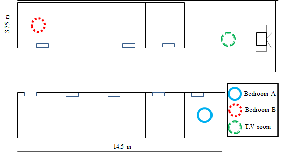
Layout of the apartments building. (Adapted by permission from Springer: Lecture Notes in Computer Science, Contextualized Hand Gesture Recognition with Smartphones, Garcia-Ceja E., Brena R., Galván-Tejada C.E., 2014, https://doi.org/10.1007/978-3-319-07491-7_13).

FIGURE 2.2: Layout of the apartments building. (Adapted by permission from Springer: Lecture Notes in Computer Science, Contextualized Hand Gesture Recognition with Smartphones, Garcia-Ceja E., Brena R., Galván-Tejada C.E., 2014, https://doi.org/10.1007/978-3-319-07491-7_13).

Table 2.1 shows the first rows of the dataset. The first column is the class. The scanid column is a unique identifier for the given Wi-Fi scan (instance). To preserve privacy, MAC addresses were converted into integer values. Every instance is composed of several rows. For example, the first instance with scanid=1 has two rows (one row per mac address). Intuitively, the same location should have similar MAC addresses across scans. From the table, we can see that at bedroomA access points with MAC address $1$ and $2$ are usually found by the device.

TABLE 2.1: First rows of Wi-Fi scans.
locationid	scanid	mac	signalstrength
bedroomA	1	1	-88.50
bedroomA	1	2	-91.00
bedroomA	2	1	-88.00
bedroomA	2	2	-90.00
bedroomA	3	1	-87.62
bedroomA	3	2	-90.00
bedroomA	4	2	-90.25
bedroomA	4	1	-90.00
bedroomA	4	3	-91.00

Since each instance is composed of several rows, we will convert our data frame into a list of lists where each inner list represents a single instance with the class (locationId), a unique id, and a data frame with the corresponding access points. The example code can be found in the script indoor_classification.R.

# Read Wi-Fi data
df <- read.csv(datapath, stringsAsFactors = F)

# Convert data frame into a list of lists.
# Each inner list represents one instance.
dataset <- wifiScansToList(df)

# Print number of instances in the dataset.
length(dataset)
#> [1] 365

# Print the first instance.
dataset[[1]]
#> $locationId
#> [1] "bedroomA"
#> 
#> $scanId
#> [1] 1
#> 
#> $accessPoints
#>   mac signalstrength
#> 1   1          -88.5
#> 2   2          -91.0

First, we read the dataset from the csv file and store it in the data frame df. To make things easier, the data frame is converted into a list of lists using the auxiliary function wifiScansToList() which is defined in the script indoor_auxiliary.R. Next, we print the number of instances in the dataset, that is, the number of lists. The dataset contains $365$ instances. The $365$ was just a coincidence, the data was not collected every day during one year but in the same day. Next, we extract the first instance with dataset[[1]]. Here, we see that each instance has three pieces of information. The class (locationId), a unique id (scanId), and a set of access points stored in a data frame. The first instance has two access points with MAC addresses $1$ and $2$. There is also information about the signal strength, though, this one will not be used.

Since we would expect that similar locations have similar MAC addresses and locations that are far away from each other have different MAC addresses, we need a distance measure that captures this notion of similarity. In this case, we cannot use the Euclidean distance on MAC addresses. Even though they were encoded as integer values, they do not represent magnitudes but unique identifiers. Each instance is composed of a set of $n$ MAC addresses stored in the accessPoints data frame. To compute the distance between two instances (two sets) we can use the Jaccard distance. This distance is based on element sets:

\[\begin{equation} j\left(A,B\right)=\frac{\left|A\cup B\right|-\left|A\cap B\right|}{\left|A\cup B\right|} \tag{2.2} \end{equation}\]

where $A$ and $B$ are sets of MAC addresses. A set is an unordered collection of elements with no repetitions. As an example, let’s say we have two sets, $S_1$ and $S_2$:

\[\begin{align*} S_1&=\{a,b,c,d,e\}\\ S_2&=\{e,f,g,a\} \end{align*}\]

The set $S_1$ has $5$ elements (letters) and $S_2$ has $4$ elements. $A \cup B$ means the union of the two sets and its result is the set of all elements that are either in $A$ or $B$. For instance, the union of $S_1$ and $S_2$ is $S_1 \cup S_2 = \{a,b,c,d,e,f,g\}$. The $A \cap B$ denotes the intersection between $A$ and $B$ which is the set of elements that are in both $A$ and $B$. In our example, $S_1 \cap S_2 = \{a,e\}$. Finally the vertical bars $||$ mean the cardinality of the set, that is, its number of elements. The cardinality of $S_1$ is $|S_1|=5$ because it has $5$ elements. The cardinality of the union of the two sets $|S_1 \cup S_2|=7$ because this set has $7$ elements.

In R, we can implement the Jaccard distance as follows:

jaccardDistance <- function(set1, set2){
  lengthUnion <- length(union(set1, set2))
  lengthIntersectoin <- length(intersect(set1, set2))
  d <- (lengthUnion - lengthIntersectoin)  / lengthUnion
  return(d)
}

The implementation is in the script indoor_auxiliary.R. Now, we can try our function! Let’s compute the distance between two instances of the same class (‘bedroomA’).

# Compute jaccard distance between instances with same class:
# (bedroomA)
jaccardDistance(dataset[[1]]$accessPoints$mac,
                dataset[[4]]$accessPoints$mac)
#> [1] 0.3333333

Now let’s try to compute the distance between instances with different classes.

# Jaccard distance of instances with different class:
# (bedroomA and bedroomB)
jaccardDistance(dataset[[1]]$accessPoints$mac,
                dataset[[210]]$accessPoints$mac)
#> [1] 0.6666667

The distance between instances of the same class was $0.33$ whereas the distance between instances of the different classes was $0.66$. So, our function is working as expected.

In the extreme case when the sets $A$ and $B$ are identical, the distance will be $0$. When there are no common elements in the sets, the distance will be $1$. Armed with this distance metric, we can now implement the $k$-NN function in R. The knn_classifier() implementation is in the script indoor_auxiliary.R. Its first argument is the dataset (the list of instances). The second argument k, is the number of nearest neighbors to use, and the last two arguments are the indices of the train and test instances, respectively. This indices are pointers to the elements in the dataset variable.

knn_classifier <- function(dataset, k, trainSetIndices, testSetIndices){
  
  groundTruth <- NULL
  predictions <- NULL
  
  for(queryInstance in testSetIndices){
    distancesToQuery <- NULL
    
    for(trainInstance in trainSetIndices){
      jd <- jaccardDistance(dataset[[queryInstance]]$accessPoints$mac,
                            dataset[[trainInstance]]$accessPoints$mac)
      distancesToQuery <- c(distancesToQuery, jd)
    }
    
    indices <- sort(distancesToQuery, index.return = TRUE)$ix
    indices <- indices[1:k]
    # Indices of the k nearest neighbors
    nnIndices <- trainSetIndices[indices]
    # Get the actual instances
    nnInstances <- dataset[nnIndices]
    # Get their respective classes
    nnClasses <- sapply(nnInstances, function(e){e[[1]]})
    prediction <- Mode(nnClasses)
    predictions <- c(predictions, prediction)
    groundTruth <- c(groundTruth,
                     dataset[[queryInstance]]$locationId)
  }
  
  return(list(predictions = predictions,
              groundTruth = groundTruth))
}

For each instance queryInstance in the test set, the knn_classifier() computes its jaccard distance to every other instance in the train set and stores those distances in distancesToQuery. Then, those distances are sorted in ascending order and the most common class among the first $k$ elements is returned as the predicted class. The function Mode() returns the most common element. Finally, knn_classifier() returns a list with the predictions for every instance in the test set and their respective ground truth class for evaluation.

Now, we can try our classifier. We will use $70\%$ of the dataset as train set and the remaining as the test set.

# Total number of instances
numberInstances <- length(dataset)
# Set seed for reproducibility
set.seed(12345)
# Split into train and test sets.
trainSetIndices <- sample(1:numberInstances,
                          size = round(numberInstances * 0.7),
                          replace = F)
testSetIndices <- (1:numberInstances)[-trainSetIndices]

The function knn_classifier() predicts the class for each test set instance and returns a list with their predictions and their ground truth classes. With this information, we can compute the accuracy on the test set which is the percentage of correctly classified instances. In this example, we set $k=3$.

# Obtain predictions on the test set.
result <- knn_classifier(dataset,
                         k = 3,
                         trainSetIndices,
                         testSetIndices)
# Calculate and print accuracy.
sum(result$predictions == result$groundTruth) /
  length(result$predictions)
#> [1] 0.9454545

Not bad! Our simple $k$-NN algorithm achieved an accuracy of $94.5\%$. Usually, it is a good idea to visualize the predictions to have a better understanding of the classifier’s behavior. Confusion matrices allow us to exactly do that. We can use the confusionMatrix() function from the caret package to generate a confusion matrix. Its first argument is a factor with the predictions and the second one is a factor with the corresponding true values. This function returns an object with several performance metrics (see next section) and the confusion matrix. The actual confusion matrix is stored in the table object.

library(caret)
cm <- confusionMatrix(factor(result$predictions),
                      factor(result$groundTruth))
cm$table # Access the confusion matrix.
#>           Reference
#> Prediction bedroomA bedroomB lobby tvroom
#> bedroomA       26        0     3      1
#> bedroomB        0       17     0      1
#> lobby           0        1    28      0
#> tvroom          0        0     0     33

The columns of the confusion matrix represent the true classes and the rows the predictions. For example, from the total $31$ instances of type ‘lobby’, $28$ were correctly classified as ‘lobby’ while $3$ were misclassified as ‘bedroomA’. Something I find useful is to plot the confusion matrix as proportions instead of counts (Figure 2.3). From this confusion matrix we see that for the class ‘bedroomB’, $94\%$ of the instances were correctly classified while $6\%$ were mislabeled as ‘lobby’. On the other hand, instances of type ‘bedroomA’ were always classified correctly.

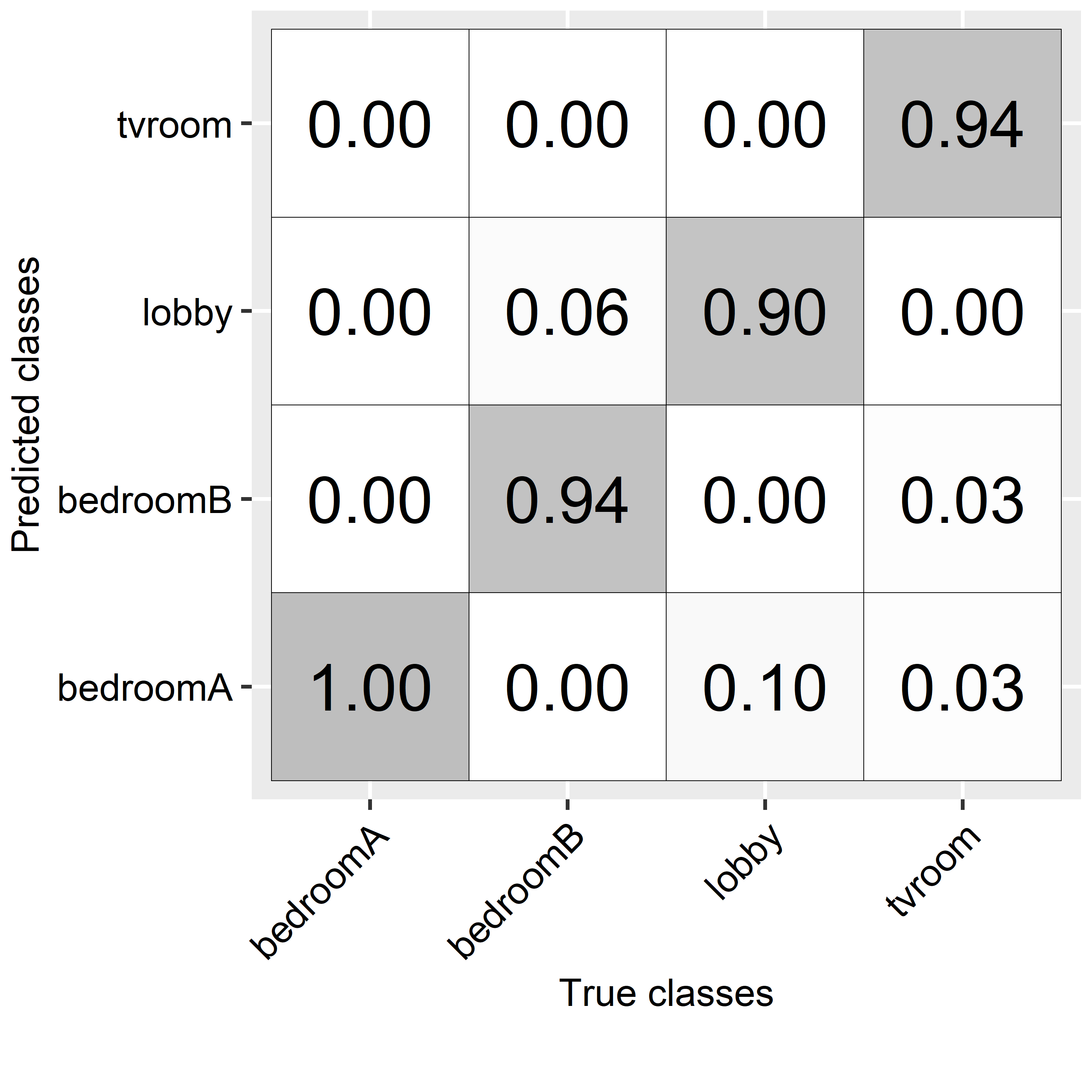
FIGURE 2.3: Confusion matrix for location predictions.

A confusion matrix is a good way to analyze the classification results per class and it helps to spot weaknesses which can be used to improve the model, for example, by extracting additional features.

2.2 Performance Metrics

Performance metrics allow us to assess the generalization performance of a model from different angles. The most common performance metric for classification is the accuracy:

\[\begin{equation} accuracy = \frac{\# \textrm{ correctly classified instances}}{\textrm{total } \# \textrm{ instances}} \tag{2.3} \end{equation}\]

In order to have a better understanding of the generalization performance of a model, it is a good practice to compute several performance metrics in addition to the accuracy. Accuracy also has some limitations, especially in highly imbalanced datasets. The following metrics provide different views of a model’s performance for the binary case (when there are only two classes). These metrics can be extended to the multi-class setting using a one vs. all approach. That is, compare each class to the remaining classes.

Before introducing the other metrics, it is convenient to define some terms:

True positives (TP): Positive examples classified as positives.
True negatives (TN): Negative examples classified as negatives.
False positives (FP): Negative examples misclassified as positives.
False negatives (FN): Positive examples misclassified as negatives.

For the binary classification case, it is you who decide which one is the positive class. For example, if your problem is about detecting falls and you have two classes: ‘fall’ and ‘nofall’, then, considering ‘fall’ as the positive class makes sense since this is the one you are most interested in detecting. The following, is a list of commonly used metrics in classification:

Recall: The proportion of positives that are classified as such. Alternative names for recall are: true positive rate, sensitivity, and hit rate. In fact, the diagonal of the confusion matrix with proportions of the indoor location example shows the recall for each class (Figure 2.3).

\[\begin{equation} recall = \frac{\textrm{TP}}{\textrm{P}} \tag{2.4} \end{equation}\]

Specificity: The proportion of negatives classified as such. It is also called the true negative rate.

\[\begin{equation} specificity = \frac{\textrm{TN}}{\textrm{N}} \tag{2.5} \end{equation}\]

Precision: The fraction of true positives among those classified as positives. Also known as the positive predictive value.

\[\begin{equation} precision = \frac{\textrm{TP}}{\textrm{TP + FP}} \tag{2.6} \end{equation}\]

F1-score: This is the harmonic mean of precision and recall.

\[\begin{equation} \textit{F1-score} = 2 \cdot \frac{\textrm{precision} \cdot \textrm{recall}}{\textrm{precision + recall}} \tag{2.7} \end{equation}\]

The confusionMatrix() function from the caret package computes several of those metrics. From our previous confusion matrix object, we can inspect those metrics by class.

cm$byClass[,c("Recall", "Specificity", "Precision", "F1")]
#>                    Recall Specificity Precision        F1
#> Class: bedroomA 1.0000000   0.9523810 0.8666667 0.9285714
#> Class: bedroomB 0.9444444   0.9891304 0.9444444 0.9444444
#> Class: lobby    0.9032258   0.9873418 0.9655172 0.9333333
#> Class: tvroom   0.9428571   1.0000000 1.0000000 0.9705882

The mean of the metrics across all classes can be computed by taking the mean for each column of the returned object:

colMeans(cm$byClass[,c("Recall", "Specificity", "Precision", "F1")])
#>    Recall Specificity   Precision          F1 
#> 0.9476318   0.9822133   0.9441571   0.9442344

2.2.1 Confusion Matrix

As briefly introduced in the previous section, a confusion matrix provides a nice way to understand the model’s predictions and spot where it made mistakes. Figure 2.4 shows a confusion matrix for the binary case. The columns represent the true classes and the rows the predicted classes. The P stands for the positive cases and the N for the negative ones. Each entry in the matrix corresponds to the TP, TN, FP, and FN. The TP and TN are the correct classifications whereas the FN and FP are the misclassifications.

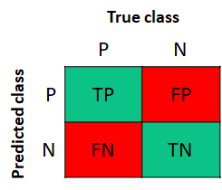
FIGURE 2.4: Confusion matrix for the binary case. P: positives, N: negatives.

Figure 2.5 shows a concrete example of a confusion matrix derived from a list of $15$ instances with their predictions and their corresponding true values (ground truth). For example, the first element in the list is a P and it was correctly classified as a P. The eight element is a P but it was misclassified as N. The associated confusion matrix for these ground truth and predicted classes is shown at the bottom.

There are $7$ true positives and $3$ true negatives. In total, $10$ instances were correctly classified (TP and TN) and $5$ were misclassified (FP and FN). From this matrix we can calculate what is the total number of true positives by taking the sum of the first column, $10$ in this case. The total number of true negatives is obtained by summing the second column, $5$ in this case. Having this information we can compute any of the previous performance metrics: accuracy, recall, specificity, precision, and F1-score.

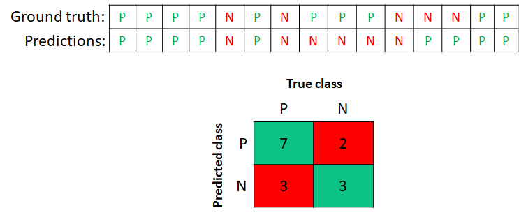
FIGURE 2.5: A concrete example of a confusion matrix for the binary case. P:positives, N:negatives.

Be aware that there is no standard that defines whether the true classes or the predicted classes go in the rows or columns, thus, you need to check for this everytime you encounter a new confusion matrix.

shiny_metrics.R This shiny app demonstrates how different performance metrics behave when the confusion matrix values change.

2.3 Decision Trees

Decision trees are powerful predictive models (especially when combining several of them, see chapter 3) used for classification and regression tasks. Here, the focus will be on classification. Each node in a tree represents partial or final decisions based on a single feature. If a node is a leaf, then it represents a final decision. A leaf is simply a terminal node, i.e, it has no children nodes. Given a feature vector representing an instance, the predicted class is obtained by testing the feature values and following the tree path until a leaf is reached. Figure 2.6 exemplifies a query instance with an unknown class (left) and a decision tree (right). To predict the class of an unknown instance, its features are evaluated starting at the root of the tree. In this case number_wheels is $4$ in the query instance so we take the left path from the root. Now, we need to evaluate weight. This time the test is false since the weight is $2300$ and we take the right path. Since this is a leaf node the final predicted class is ‘truck’. Usually, small trees are preferable (small depth) because they are easier to visualize and interpret and are less prone to overfitting. The example tree has a depth of 2. Had the number of wheels been $2$ instead of $4$, then testing the weight feature would not have been necessary.

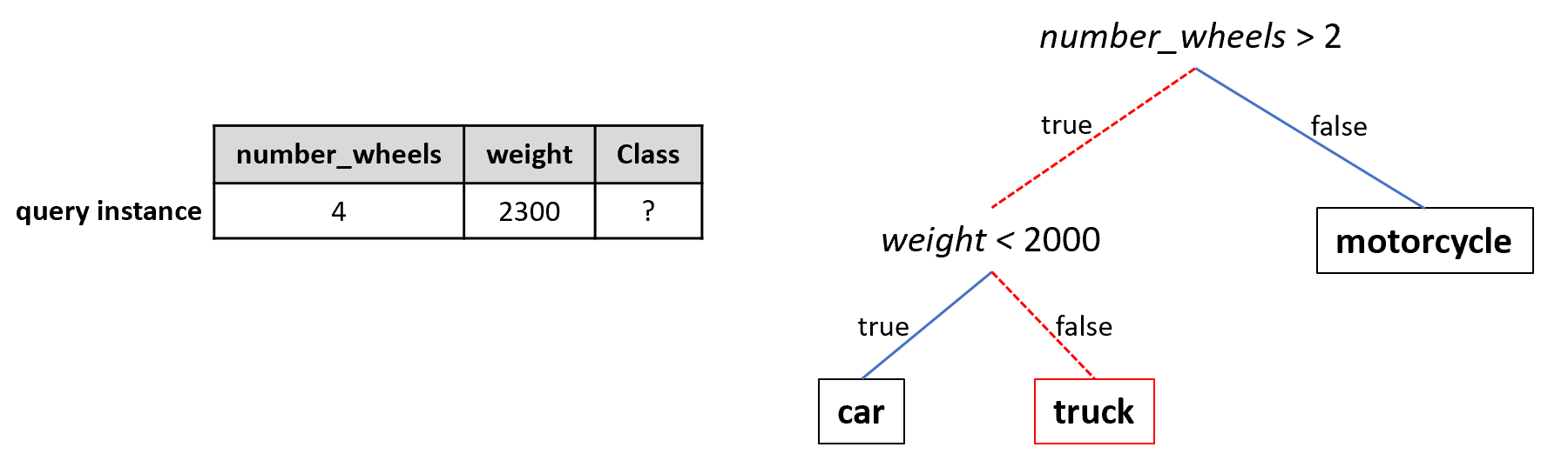
FIGURE 2.6: Example decision tree. The query instance is classified as truck by this tree.

As shown in the example, decision trees are easy to interpret and the final result can be explained by just following the path. Now let’s see how these decision trees are learned from data. Consider the following artificial concert dataset (Figure 2.7).

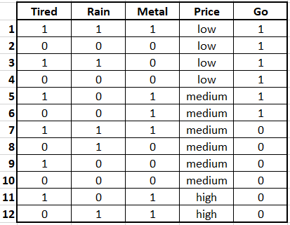
FIGURE 2.7: Concert dataset.

The first four variables are features and the last column is the class. The class is the decision whether or not we should go to a music concert based on the other variables. In this case, all variables are binary except Price which has three possible values: low, medium, and high.

Tired: Indicates whether the person is tired or not.
Rain: Whether it is raining or not.
Metal: Indicates whether this is a heavy metal concert or not.
Price: Ticket price.
Go: The decision of whether to go to the music concert or not.

The main question when building a tree is which feature should be at the root (top). Once you answer this question, you may need to grow the tree by adding another feature (node) as one of the root’s children. To decide which new feature to add you need to answer the same first question: “What feature should be at the root of this subtree?”. This is a recursive definition! The tree keeps growing until you reach a leaf node, there are no more features to select from, or you have reached a predefined maximum depth.

For the concert dataset we need to find which is the best variable to be placed at the root. Let’s suppose we need to choose between Price and Metal. Figure 2.8 shows these two possibilities.

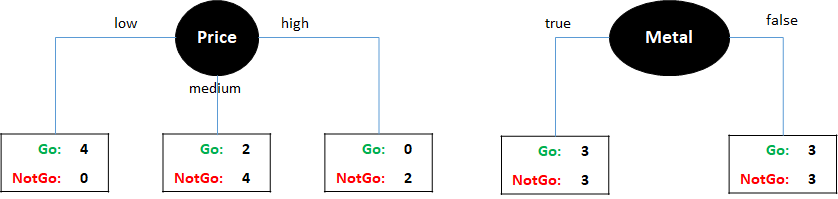
FIGURE 2.8: Two example trees with one variable split by Price (left) and Metal (right).

If we select Price, there are three possible subnodes, one for each value: low, medium, and high. If Price is low then four instances fall into this subtree (the first four from the table). For all of them, the value of Go is $1$. If Price is high, two instances fall into this category and their Go value is $0$, thus if the price is high then you should not go to the concert according to this data. There are six instances for which the Price value is medium. From those, two of them have Go=1 and the remaining four have Go=0. For cases when the price is low or high we can arrive at a solution. If the price is low then go to the concert, if the price is high then do not go. However, if the price is medium it is still not clear what to do since this subnode is not pure. That is, the labels of the instances are mixed: two with an output of $1$ and four with an output of $0$. In this case we can try to use another feature to decide and grow the tree but first, let’s look at what happens if we decide to use Metal as the first feature at the root. In this case, we end up with two subsets with six instances each. And for each subnode, what decision should we take is still not clear because the output is ‘mixed’ (Go: 3, NotGo: 3). At this point we would need to continue growing the tree below each subnode.

Intuitively, it seems like Price is a better feature since its subnodes are more pure. Then we can use another feature to split the instances whose Price is medium. For example, using the Metal variable. Figure 2.9 shows how this would look like. Since one of the subnodes of Metal is still not pure we can further split it using the Rain variable, for example. At this point, we can not split any further. Note that the Tired variable was never used.

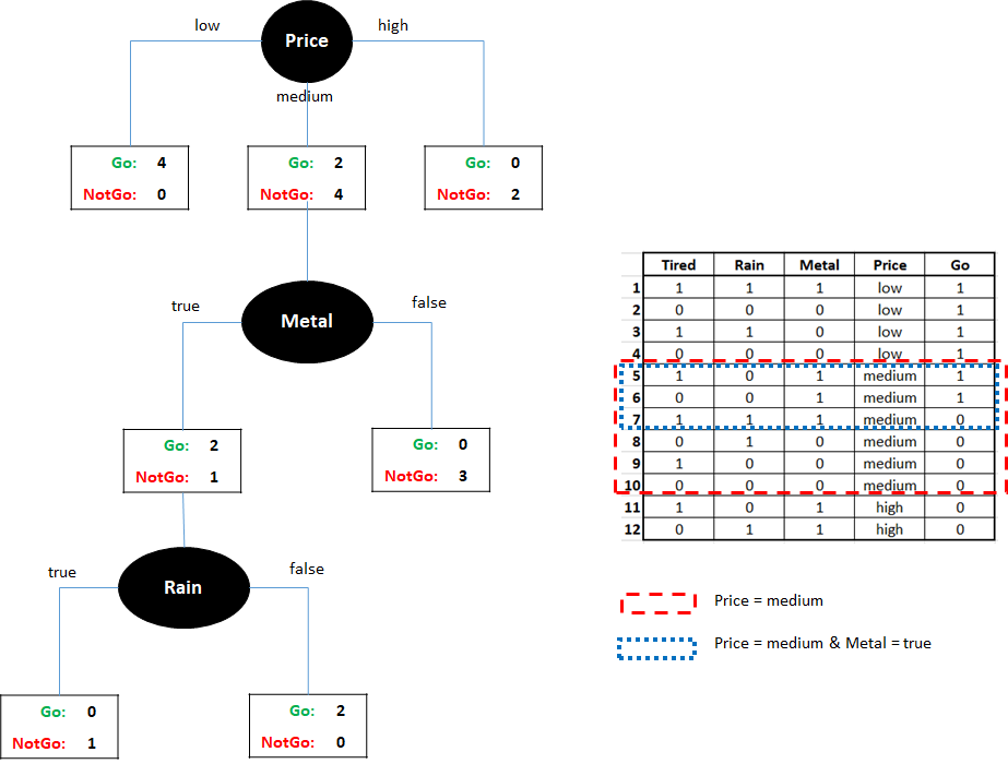
FIGURE 2.9: Tree splitting example. Left:tree splits. Right:Highlighted instances when splitting by Price and Metal.

So far, we have chosen the root variable based on which one looks more pure but to automate the process, we need a way to measure this purity in a quantitative manner. One way to do that is by using the entropy. Entropy is a measure of uncertainty from information theory. It is $0$ when there is no uncertainty and $1$ when there is complete uncertainty. The entropy of a discrete variable $X$ with values $x_1\dots x_n$ and probability mass function $P(X)$ is:

\[\begin{equation} H(X) = -\sum_{i=1}^n{P(x_i)log P(x_i)} \tag{2.8} \end{equation}\]

Take for example a fair coin with probability of heads and tails = $0.5$ each. The entropy for that coin is:

\[\begin{equation*} H(X) = - (0.5)log(0.5) + (0.5)log(0.5) = 1 \end{equation*}\]

Since we do not know what will be the result when we drop the coin, the entropy is maximum. Now consider the extreme case when the coin is biased such that the probability of heads is $1$ and the probability of tails is $0$. The entropy in this case is zero:

\[\begin{equation*} H(X) = - (1)log(1) + (0)log(0) = 0 \end{equation*}\]

If we know that the result is always going to be heads, then there is no uncertainty when the coin is dropped. The entropy of $p$ positive examples and $n$ negative examples is:

\[\begin{equation} H(p, n) = - (\frac{p}{p+n})log(\frac{p}{p+n}) + (\frac{n}{p+n})log(\frac{n}{p+n}) \tag{2.9} \end{equation}\]

Thus, we can use this to compute the entropy for the three possible values of Price with respect to the class. The positives are the instances where Go=1 and the negatives are the instances where Go=0:

\[\begin{equation*} H_{price=low}(4, 0) = - (\frac{4}{4+0})log(\frac{4}{4+0}) + (\frac{0}{4+0})log(\frac{0}{4+0}) = 0 \end{equation*}\]

\[\begin{equation*} H_{price=medium}(2, 4) = - (\frac{2}{2+4})log(\frac{2}{2+4}) + (\frac{4}{2+4})log(\frac{4}{2+4}) = 0.918 \end{equation*}\]

\[\begin{equation*} H_{price=high}(0, 2) = - (\frac{0}{0+2})log(\frac{0}{0+2}) + (\frac{2}{0+2})log(\frac{2}{0+2}) = 0 \end{equation*}\]

The average of those three can be calculated by taking into account the number of corresponding instances for each value and the total number of instances ($12$):

\[\begin{equation*} meanH(price) = (4/12)(0) + (6/12)(0.918) + (2/12)(0) = 0.459 \end{equation*}\]

Before deciding to split on Price the entropy of the entire dataset is $1$ since there are six positive and negative examples:

\[\begin{equation*} H(6,6) = 1 \end{equation*}\]

Now we can compute the information gain for Price. Intuitively, the information gain tells you how powerful this variable is at dividing the instances based on their class, that is, how much you are learning:

\[\begin{equation*} infoGain(Price) = 1 - meanH(Price) = 1 - 0.459 = 0.541 \end{equation*}\]

Since you want to learn fast, you want your root node to be the one with the highest information gain. For the rest of the variables the information gain is:

$infoGain(Tired) = 0$

$infoGain(Rain) = 0.020$

$infoGain(Metal) = 0$

The highest information gain is produced by Price, thus, it is selected as the root node. Then, the process continues recursively for each branch but excluding Price. Since branches with values low and high are already done, we only need to further split medium. Sometimes it is not possible to have completely pure nodes like with low and high. This can happen for example, when there are no more attributes left or when two or more instances have the same feature values but different labels. In those situations the final prediction is the most common label (majority vote).

There exist many implementations of decision trees. Some implementations compute variable importance using the entropy (as shown here) but others use the Gini index, for example. Each implementation also treats numeric variables in different ways. Pruning the tree using different techniques is also common in order to reduce its size.

Some of the most common implementations are C4.5 trees (Quinlan 2014) and CART (Steinberg and Colla 2009). The later is implemented in the rpart R package (Therneau and Atkinson 2019) which will be used in the following section to build a model that predicts physical activities from smartphones sensor data.

2.3.1 Activity Recognition with Smartphones

smartphone_activities.R

As mentioned in the introduction, an example of behavior is an observable physical activity. We can infer what physical activity someone is doing by looking at her/his body movements. Observing physical activities can provide useful behavioral and contextual information about someone. This can also be used as a proxy to, for example, infer someone’s health condition by detecting deviations in activity patterns.

Nowadays, most smartphones come with a tri-axial accelerometer sensor. This sensor measures gravitational forces from the $x$, $y$, and $z$ axes. This information can be used to capture movement patterns from the user and automate the process of monitoring the type of physical activity being performed.

In this section, we will use decision trees to automatically classify physical activities from acceleration data. We will use the WISDM dataset⁵ and from now on, I will refer to it as the SMARTPHONE ACTIVITIES dataset. It contains acceleration recordings that were collected with a smartphone and was made available by Kwapisz, Weiss, and Moore (2010). The dataset has $6$ different activities: ‘walking’, ‘jogging’, ‘walking upstairs’, ‘walking downstairs’, ‘sitting’ and ‘standing’. The data were collected by $36$ volunteers with an Android phone located in their pant’s pocket and with a sampling rate of $20$ Hz ($1$ sample every $50$ milliseconds).

The dataset contains two types of files. One with the raw accelerometer data and the other one after feature extraction. Figure 2.10 shows the first $10$ lines of the raw accelerometer values of the first file. The first column is the id of the user that collected the data and the second column is the class. The third column is the timestamp and the remaining columns are the $x$, $y$, and $z$ accelerometer values, respectively.

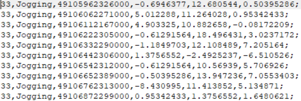
FIGURE 2.10: First 10 lines of raw accelerometer data.

Usually, classification models are not trained with the raw data but with feature vectors extracted from the raw data. Feature vectors have the advantage of being more compact, thus, making the learning phase more efficient. For activity recognition, the feature extraction process consists of defining a moving window of size $w$ that starts at position $i$. At the beginning, $i$ is the index pointing to the first accelerometer readings. Then, $n$ statistical features are computed on the elements covered by the window such as mean, standard deviation, $0$-crossings, etc. This will produce a $n$-dimensional feature vector and the process is repeated by moving the window $s$ steps forward. Typical values of $s$ are such that the overlap between the previous window position and the next one is about $30\%$ to $50\%$. An overlap of $0$ is also typical, that is, $s = w$. Figure 2.11 depicts the process.

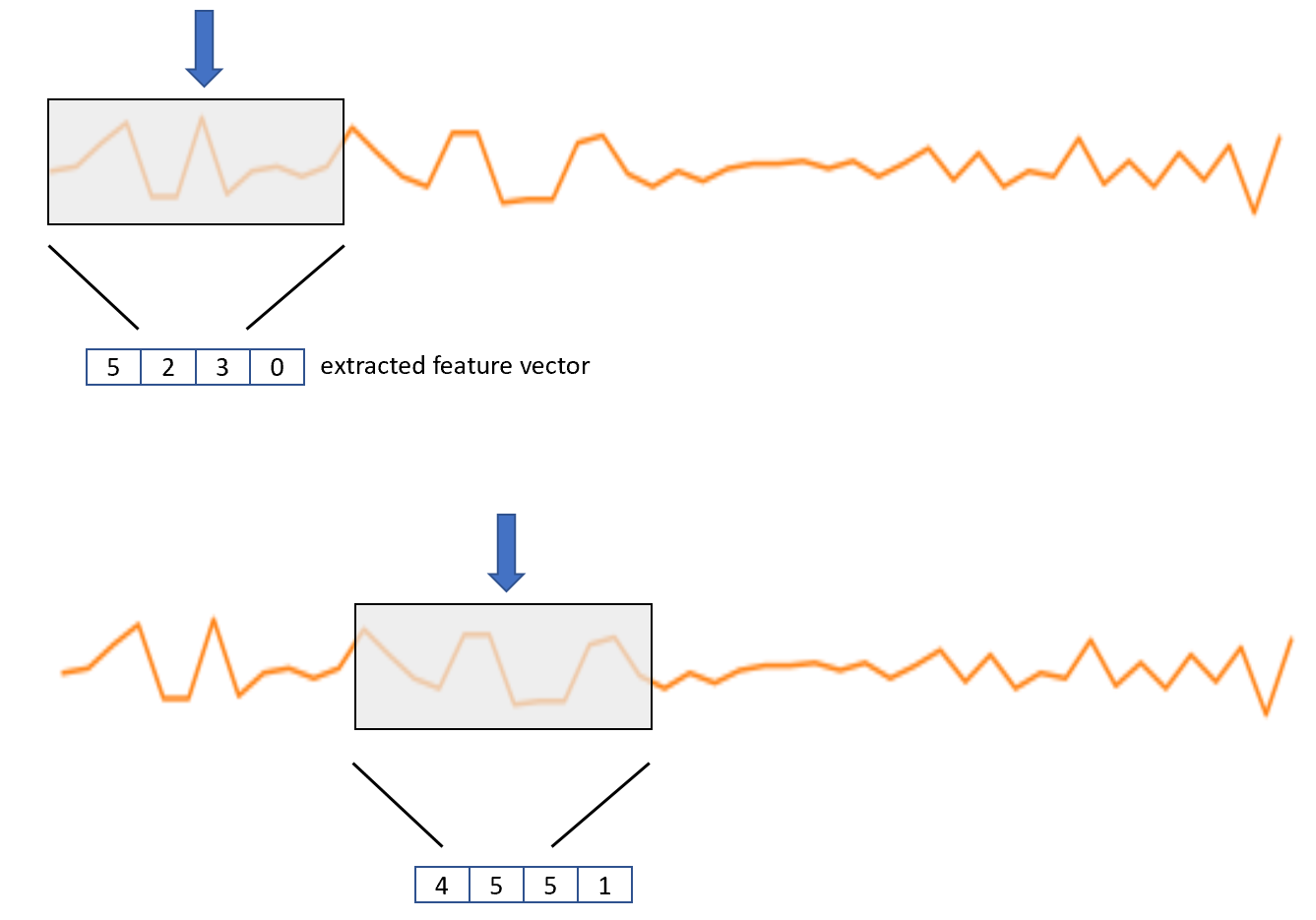
FIGURE 2.11: Moving window for feature extraction.

Once we have the set of feature vectors and their associated class labels, we can use them to train a classifier and make predictions on new data (Figure 2.12).

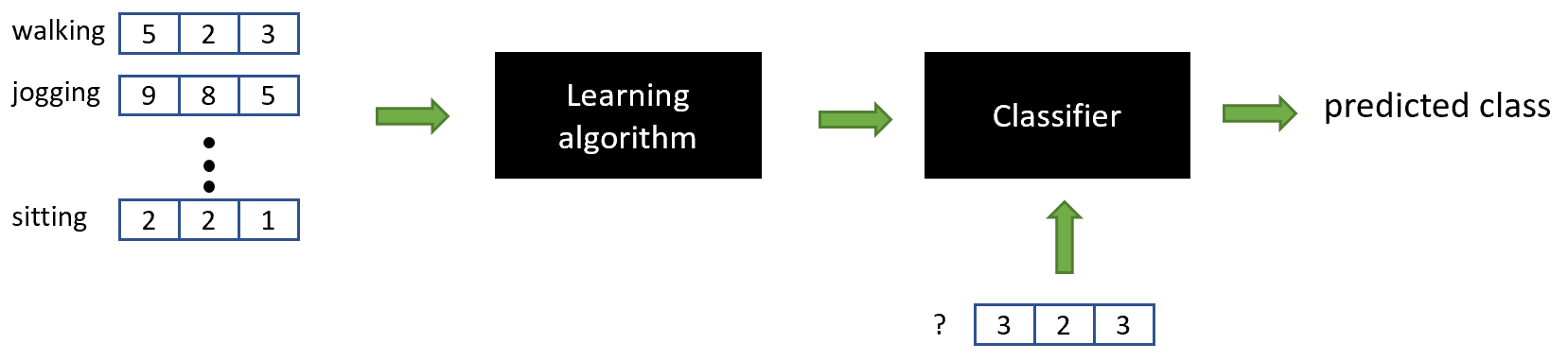
FIGURE 2.12: The extracted feature vectors are used to train a classifier.

For this example, we will use the file with features already extracted. The authors used windows of $10$ seconds which is equivalent to $200$ observations given the $20$ Hz sampling rate and they used $0\%$ overlap. From each window, they extracted $43$ features such as the mean, standard deviation, absolute deviations, etc.

Let’s read and print the first rows of the dataset. The script for this section is smartphone_activities.R. The data frame has several columns, but we only print the first five features and the class which is stored in the last column.

# Read data.
df <- read.csv(datapath,stringsAsFactors = F)

# Some code to clean the dataset.
# (cleaning code not shown here).

# Print first rows of the dataset.
head(df[,c(1:5,40)])

#>     X0   X1   X2   X3   X4    class
#> 1 0.04 0.09 0.14 0.12 0.11  Jogging
#> 2 0.12 0.12 0.06 0.07 0.11  Jogging
#> 3 0.14 0.09 0.11 0.09 0.09  Jogging
#> 4 0.06 0.10 0.09 0.09 0.11  Walking
#> 5 0.12 0.11 0.10 0.08 0.10  Walking
#> 6 0.09 0.09 0.10 0.12 0.08  Walking
#> 7 0.12 0.12 0.12 0.13 0.15 Upstairs
#> 8 0.10 0.10 0.10 0.10 0.11 Upstairs
#> 9 0.08 0.07 0.08 0.08 0.05 Upstairs

Our aim is to predict the class based on all the numeric features. We will use the rpart package (Therneau and Atkinson 2019) which implements classification and regression trees. We will assess the performance of the decision tree with $10$-fold cross-validation. We can use the sample() function to generate the folds. This function will sample $n$ integers from $1$ to $k$ where $n$ is the number of rows in the data frame.

# Package with implementations of decision trees.
library(rpart)

# Set seed for reproducibility.
set.seed(1234)

# Define the number of folds.
k <- 10

# Generate folds.
folds <- sample(k, size = nrow(df), replace = TRUE)

# Print first 10 values.
head(folds)
#> [1] 10  6  5  9  5  6

The folds variable stores the fold each instance belongs to. For example, the first instance belongs to fold $10$, the second instance belongs to fold $6$, and so on. We can now generate our test and train sets. We will iterate $k=10$ times. For each iteration $i$, the test set is built using the instances that belong to fold $i$ and the train set will be composed of the remaining instances (those that do not belong to fold $i$). Next, the rpart() function is used to train the decision tree with the train set. By default, rpart() performs $10$-fold cross-validation internally. To avoid this, we set the parameter xval = 0. Then, we can use the trained model to obtain the predictions on the test set with the generic predict() function. The ground truth classes and the predictions are stored so the performance metrics can be computed.

# Variable to store ground truth classes.
groundTruth <- NULL

# Variable to store the classifier's predictions.
predictions <- NULL

for(i in 1:k){
  
  trainSet <- df[which(folds != i), ]
  testSet <- df[which(folds == i), ]
  
  # Train the decision tree
  treeClassifier <- rpart(class ~ .,
                          trainSet, xval=0)
  
  # Get predictions on the test set.
  foldPredictions <- predict(treeClassifier,
                             testSet, type = "class")
  
  predictions <- c(predictions,
                   as.character(foldPredictions))
  
  groundTruth <- c(groundTruth,
                   as.character(testSet$class))
}

The first argument of the rpart() function is class ~ . which is a formula that instructs the method to use the class column as the class. The ~ . means “use all the remaining columns as features”. Now, we can use the confusionMatrix() function to compute the performance metrics and the confusion matrix.

cm <- confusionMatrix(as.factor(predictions),
                      as.factor(groundTruth))

# Print accuracy
cm$overall["Accuracy"]
#> Accuracy 
#> 0.7895903 

# Print performance metrics per class.
cm$byClass[,c("Recall", "Specificity", "Precision", "F1")]
#>                      Recall Specificity Precision        F1
#> Class: Downstairs 0.2821970   0.9617587 0.4434524 0.3449074
#> Class: Jogging    0.9612308   0.9601898 0.9118506 0.9358898
#> Class: Sitting    0.8366013   0.9984351 0.9696970 0.8982456
#> Class: Standing   0.8983740   0.9932328 0.8632812 0.8804781
#> Class: Upstairs   0.2246835   0.9669870 0.4733333 0.3047210
#> Class: Walking    0.9360884   0.8198981 0.7642213 0.8414687

# Print overall metrics across classes.
colMeans(cm$byClass[,c("Recall", "Specificity",
                       "Precision", "F1")])
#>     Recall Specificity   Precision          F1 
#>  0.6898625   0.9500836   0.7376393   0.7009518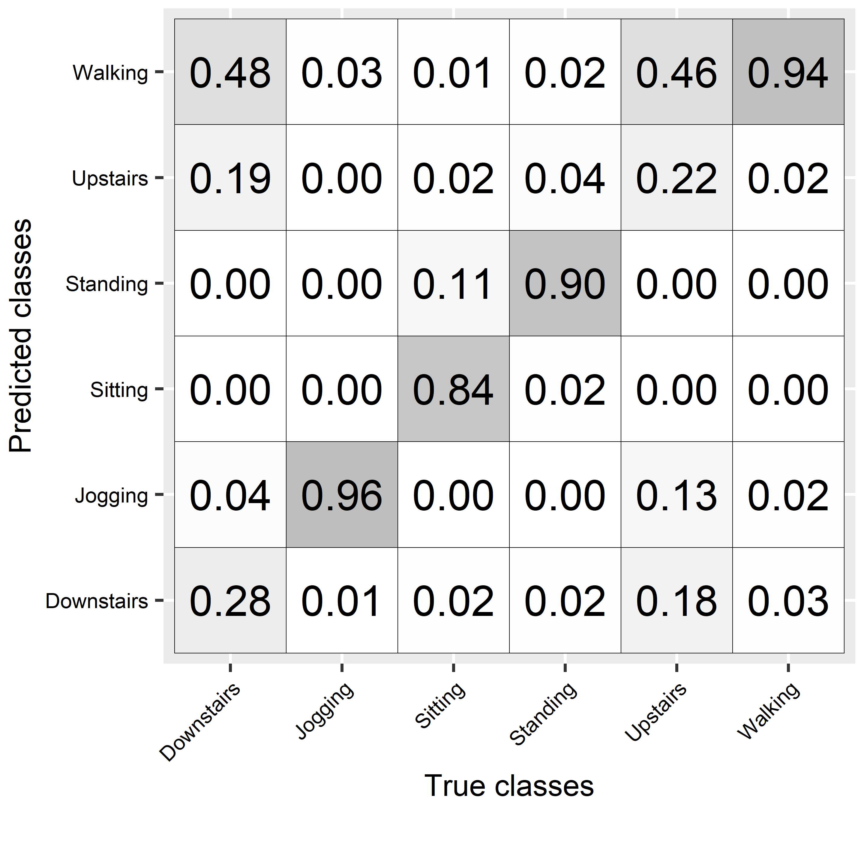

FIGURE 2.13: Confusion matrix for activities’ predictions.

The overall accuracy was $78\%$ and by looking at the individual performance metrics, some classes had low scores like ‘walking downstairs’ and ‘walking upstairs’. From the confusion matrix (Figure 2.13), it can be seen that those two activities were often confused with each other but also with the ‘walking’ activity. The package rpart.plot (Milborrow 2019) can be used to plot the resulting tree (Figure 2.14).

library(rpart.plot)
# Plot the tree from the last fold.
rpart.plot(treeClassifier, fallen.leaves = F,
           shadow.col = "gray", legend.y = 1)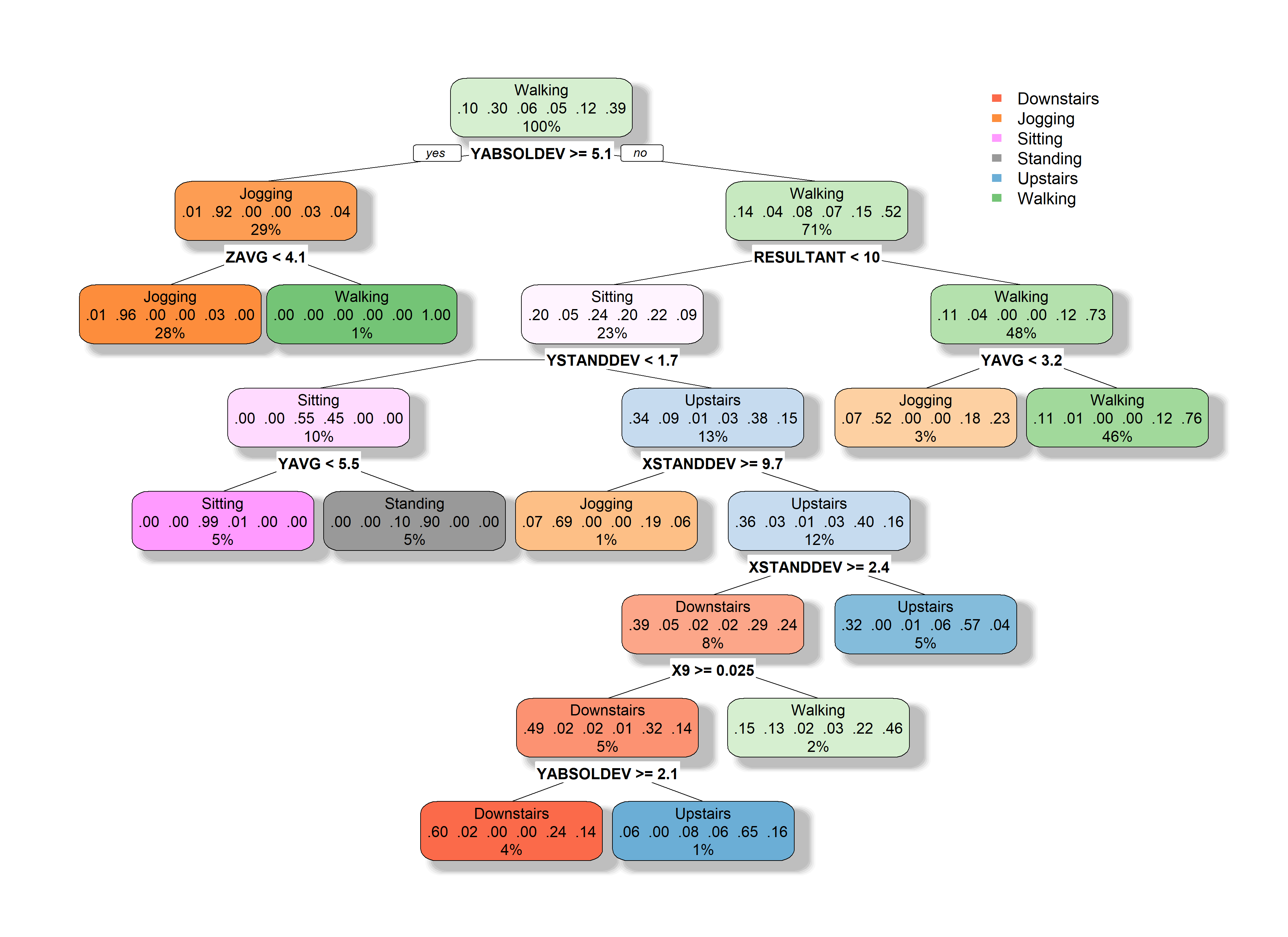

FIGURE 2.14: Resulting decision tree.

The fallen.leaves = F argument prevents the leaves to be plotted at the bottom. This is useful if the tree has many nodes. Each node shows the predicted class, the predicted probability of each class, and the percentage of observations in the node. The plot also shows the feature used for each split. We can see that the YABSOLDEV variable is at the root thus, it had the highest information gain with the initial set of instances. At the root of the tree, before looking at any of the features, the predicted class is ‘Walking’. This is because its prior probability is the highest one ($\approx 0.39$), that is, it’s the most common activity present in the dataset. So, if we didn’t have any other information, our best bet would be to predict the most frequent activity.

# Prior probabilities.
table(trainSet$class) / nrow(trainSet)
#> Downstairs    Jogging    Sitting   Standing   Upstairs    Walking 
#> 0.09882885 0.29607561 0.05506472 0.04705157 0.11793713 0.38504212

These results look promising, but they can still be improved. In the next chapter, I will show you how to improve these results with Ensemble Learning which is a method that is used to aggregate many models.

2.4 Naive Bayes

Naive Bayes is yet another type of classifier. This one is based on Bayes’ rule. The name Naive is because this method assumes that the features are independent. In the previous section we learned that decision trees are built recursively. Trees are built by first selecting a feature to be at the root and then, the root is split into subnodes and so on. How those subnodes are chosen depends on their parent node. With Naive Bayes, features don’t need information about other features, thus, the parameters for each feature can be learned in parallel.

To demonstrate how Naive Bayes works I will use the SMARTPHONE ACTIVITIES dataset as in the previous section. For any given query instance, the aim is to predict its most likely class based on the accelerometer features. For a new query instance, we want to estimate its class based on the features that we have observed. Let’s say we want to know what is the probability that the query instance belongs to the class ‘Walking’. This can be formulated as follows:

\[\begin{equation*} P(C=\textit{Walking} | f_1,\dots ,f_n). \end{equation*}\]

This reads as the conditional probability that the class is ‘Walking’ given the observed evidence. For each instance, the evidence that we can observe are its features $f_1, \dots ,f_n$. In this dataset, each instance has $39$ features. If we want to estimate the most likely class, all we need to do is to compute the conditional probability for each class and return the highest one:

\[\begin{equation} y = \operatorname*{arg max}_{k \in \{1, \dots ,K\}} P(C_k | f_1,\dots ,f_n) \tag{2.10} \end{equation}\]

where $K$ is the total number of possible classes. The $\text{arg max}$ notation means: Evaluate the right hand expression for every class $k$ and return the $k$ that resulted with the maximum probability. If instead of arg max we had max (without the arg) that would mean to return the actual maximum probability instead of the class $k$.

Now let’s see how we can compute $P(C_k | f_1,\dots ,f_n)$. To compute a conditional probability we can use Bayes’ rule:

\[\begin{equation} P(H|E) = \frac{P(H)P(E|H)}{P(E)} \tag{2.11} \end{equation}\]

Let’s dissect that formula:

$P(H|E)$ is called the posterior and it is the probability of the hypothesis $H$ given the observed evidence $E$. In our example, the hypothesis can be that $C=Walking$ and the evidence consists of the measured features. This is the probability that ultimately we want to estimate for each class and pick the class with the highest probability.
$P(H)$ is called the prior. This is the probability of a hypothesis happening without having any evidence. In our example, this translates into the probability that an instance belongs to a particular class without looking at its features. In practice, this is estimated from the class counts in the training set. Suppose the training set consists of $100$ instances and from those, $80$ are of type ‘Walking’ and $20$ are of type ‘Jogging’. Then, the prior probability for ‘Walking’ is $P(C=Walking)=80/100=0.8$ and the prior for ‘Jogging’ is $P(C=Jogging)=20/100=0.2$.
$P(E)$ is the probability of the evidence. Since this one doesn’t depend on the class we don’t need to compute it. This can be thought of as a normalization factor. When choosing the final class we only need to select the one with the highest score, so there is no need to normalize them into proper probabilities between $0$ and $1$.
$P(E|H)$ is called the likelihood. For numerical variables we can estimate this using a Gaussian probability density function. This sounds intimidating! but all we need to do is to compute the mean and standard deviation for each feature-class pair and plug them in the probability density function (pdf). The formula for a Gaussian (also called normal) pdf is:

\[\begin{equation} f(x) = \frac{1}{{\sigma \sqrt {2\pi } }}e^{ - \left( {x - \mu } \right)^2 / 2 \sigma ^2 } \tag{2.12} \end{equation}\]

where $\mu$ is the mean and $\sigma$ is the standard deviation.

Suppose that for some feature $f1$ when the class is ‘Walking’, its mean is $5$ and its standard deviation is $3$. That is, we filter the train set and only select those instances with class ‘Walking’ and compute the mean and standard deviation for feature $f1$. Figure 2.15 shows how its pdf looks like.

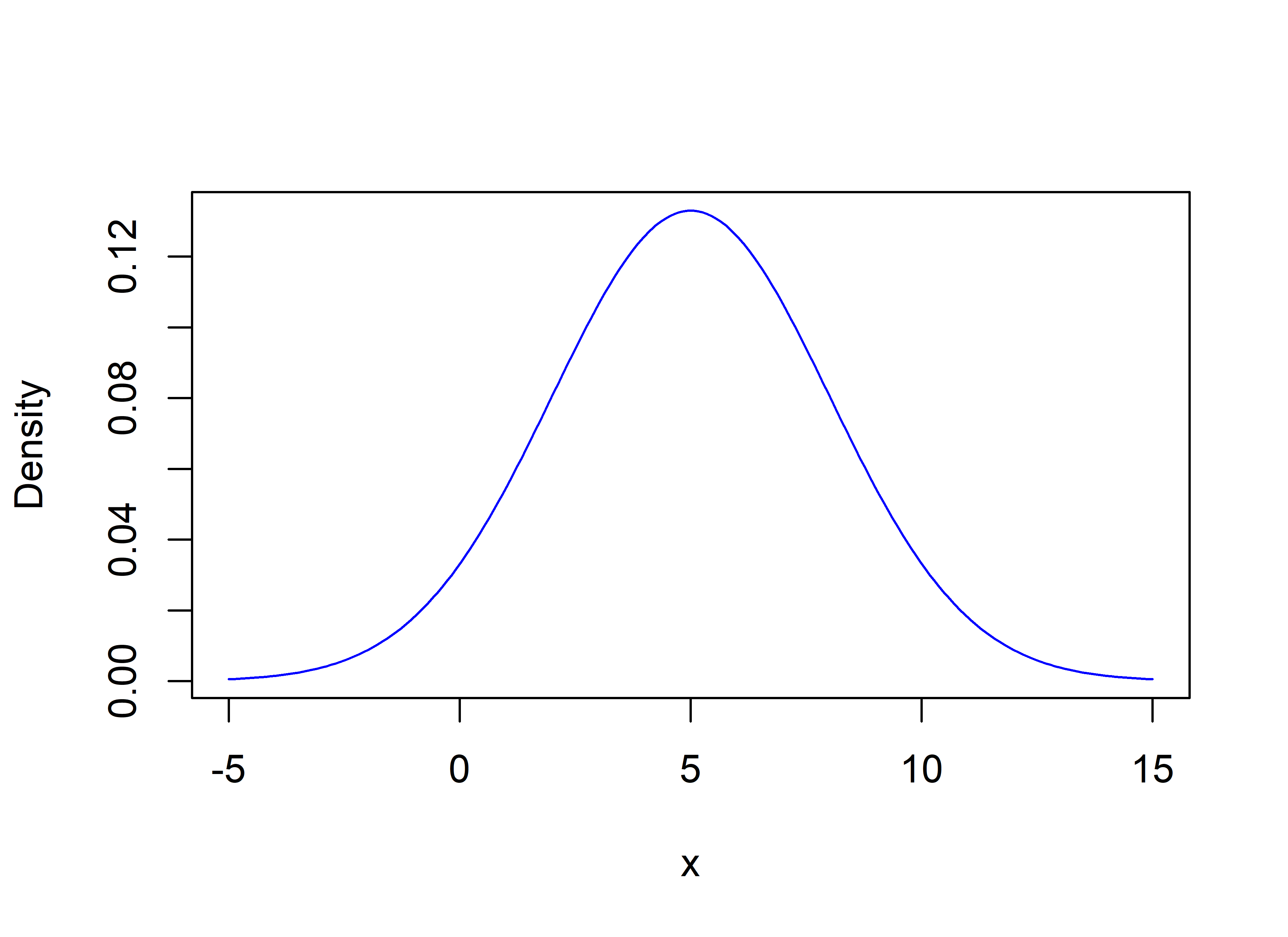
FIGURE 2.15: Gaussian probability density function with mean 5 and standard deviation 3.

If we have a query instance with a feature $f_1 = 1.7$, we can compute its likelihood given the ‘Walking’ class $P(f_1=1.7|C=Walking)$ with equation (2.12) by plugging $x=1.7$, $\mu=5$, and $\sigma=3$. In R, the function dnorm() implements the normal pdf.

dnorm(x=1.7, mean = 5, sd = 3)
#> [1] 0.07261739

In Figure 2.16 the solid circle shows the likelihood when $x=1.7$.

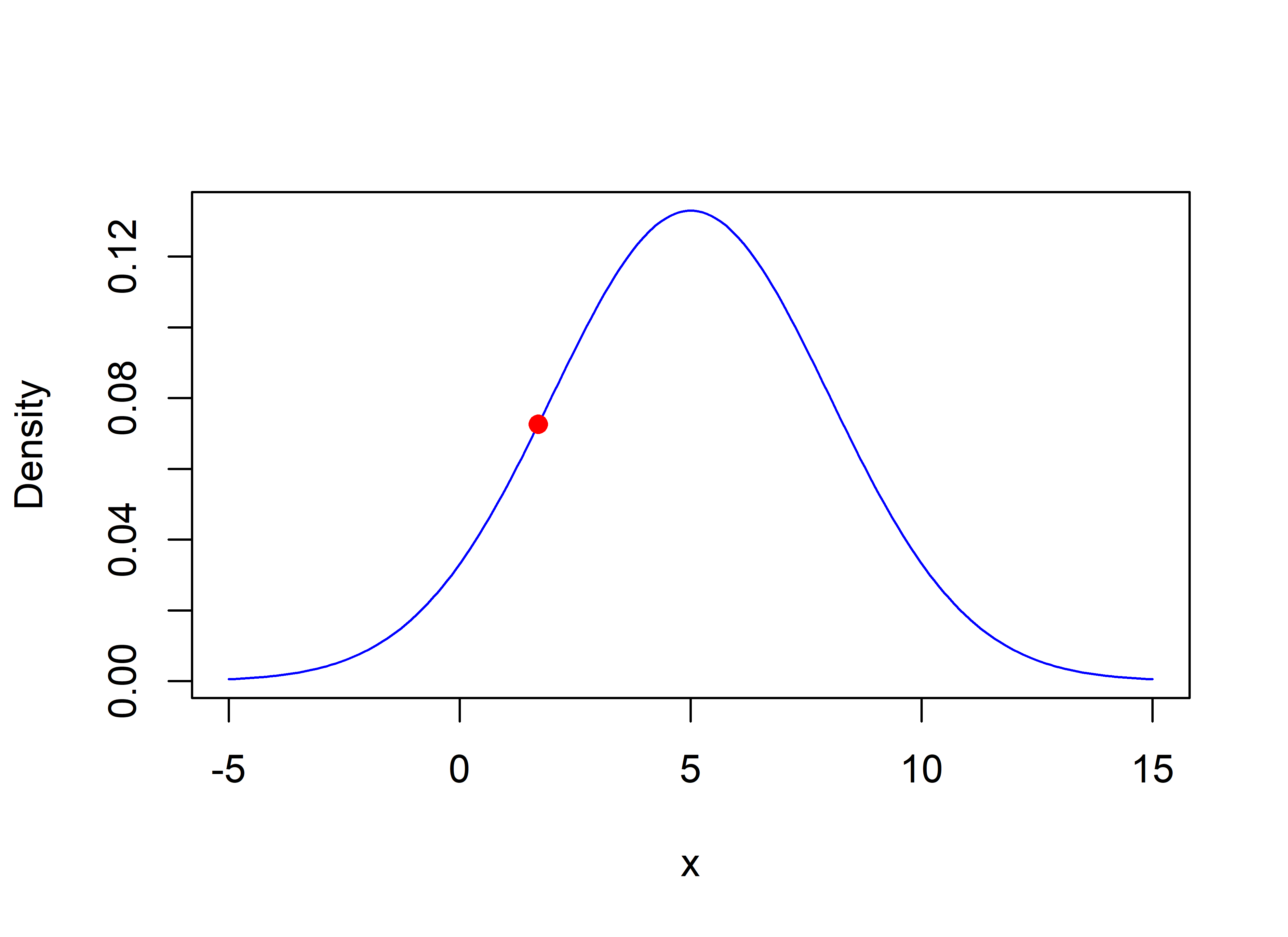
FIGURE 2.16: Likelihood (0.072) when x=1.7.

If we have more than one feature we need to compute the likelihood for each and take their product: $P(f_1|C=Walking)*P(f_2|C=Walking)*\dots*P(f_n|C=Walking)$. Each feature and class pair has its own $\mu$ and $\sigma$ parameters. Thus, Naive Bayes requires to learn $K*F*2$ parameters for the $P(E|H)$ part plus $K$ parameters for the priors $P(H)$. $K$ is the number of classes, $F$ is the number of features, and the $2$ stands for the mean and standard deviation.

We have seen how we can compute $P(C_k|f_1, \dots ,f_n)$ using Baye’s rule by calculating the prior $P(H)$ and $P(E|H)$ which is the product of the likelihoods for each feature. If we substitute Bayes’s rule (omitting the denominator) in equation (2.10) we get our Naive Bayes classifier:

\[\begin{equation} y = \operatorname*{arg max}_{k \in \{1, \dots ,K\}} P(C_k) \prod_{i=1}^{F} P(f_i | C_k) \tag{2.13} \end{equation}\]

In the following section we will implement our own Naive Bayes algorithm in R and test it on the SMARTPHONE ACTIVITIES dataset. Then, we will compare our implementation with that of the well known e1071 package (Meyer et al. 2019).

Naive Bayes works well with missing values since the features are independent. At prediction time, if an instance has one or more missing values then, those features are just ignored and the posterior probability is computed based only on the available variabels. Another advantage of the feature independence assumption is that feature selection algorithms run very fast with Naive Bayes. When building a predictive model, not all features may provide useful information and some features may even degrade the performance. Feature selection algorithms aim to find the best set of features and some of them need to try a huge number of feature combinations. With Naive Bayes, the parameters only need to be learned once and then different combinations of features can be evaluated by omitting the ones that are not used. With decision trees, for example, we would need to build entire new trees every time we want to try different input features.

Here, we have shown how we can use a Gaussian pdf to compute the likelihood $P(E|H)$ when the features are numeric. This assumes that the features have a normal distribution. However, this is not always the case. In practice, Naive Bayes can work really well even if that assumption is not met. Furthermore, nothing prevents us from using another distribution to estimate the likelihood or even defining a specific distribution for each feature. For categorical variables, $P(E|H)$ is estimated using the frequencies of the feature values.

2.4.1 Activity Recognition with Naive Bayes

naive_bayes.R

It’s time to implement Naive Bayes. To keep it simple, first we will go through a step by step example using a single feature. Then, we will implement a function to train a Naive Bayes classifier for the case of multiple features.

Let’s assume we have already split the data into train and test sets. The complete code is in the script naive_bayes.R. We will only use the feature RESULTANT which corresponds to the acceleration magnitude of the three axes of the accelerometer sensor. The following code snippet prints the first rows of the train set. The RESULTANT feature is in column $39$ and the class is the last column ($40$).

head(trainset[,c(39:40)])
#>      RESULTANT    class
#> 1004     11.14  Walking
#> 623       1.24 Upstairs
#> 2693      9.90 Standing
#> 934      10.44 Upstairs
#> 4496     10.43  Walking
#> 2948     15.28  Jogging

First, we compute the prior probabilities for each class in the train set and store them in the variable priors. This corresponds to the $P(C_k)$ part in equation (2.13).

# Compute prior probabilities.
priors <- table(trainset$class) / nrow(trainset)

# Print the table of priors.
priors

#> Downstairs    Jogging    Sitting   Standing   Upstairs 
#> 0.09622990 0.30266280 0.05721065 0.04640127 0.11521223 
#>    Walking 
#> 0.38228315

We can access each prior by name like this:

# Get the prior for "Jogging".
priors["Jogging"]
#>   Jogging 
#> 0.3026628

This means that $30\%$ of the instances in the train set are of type ‘Jogging’. Now we need to compute the $P(f_i|C_k)$ part from equation (2.13). In R, we can define a method to compute the probability density function from equation (2.12) as:

# Probability density function of normal distribution.
f <- function(x, m, s){
  (1 / (sqrt(2*pi)*s)) * exp(-((x-m)^2) / (2 * s^2))
}

It’s first argument x is the input value. The second argument m is the mean, and the last argument s is the standard deviation. For illustration purposes we are defining this function manually but remember that this pdf is already implemented with the base dnorm() function.

According to equation (2.13) we need to compute $P(f_i|C_k)$ for each feature $i$ and class $k$. Let’s assume there are only two classes, ‘Walking’ and ‘Jogging’. Thus, we need to compute the mean and standard deviation for each, and for the feature RESULTANT (column $39$).

# Compute the mean and sd of
# the feature RESULTANT (column 39)
# when the class = "Standing".
mean.standing <- mean(trainset[which(trainset$class == "Standing"), 39])
sd.standing <- sd(trainset[which(trainset$class == "Standing"), 39])

# Compute mean and sd when
# the class = "Jogging".
mean.jogging <- mean(trainset[which(trainset$class == "Jogging"), 39])
sd.jogging <- sd(trainset[which(trainset$class == "Jogging"), 39])

Print the means:

mean.standing
#> [1] 9.405795
mean.jogging
#> [1] 13.70145

Note that the mean value for ‘Jogging’ is higher for this feature. This was expected since this feature captures the overall movement across all axes. Now we have everything we need to start making predictions on new instances. We have the priors and we have the means and standard deviations for each feature-class pair.

Let’s select the first instance from the test set and try to predict its class.

# Select a query instance from the test set.
query <- testset[1,] # Select the first one.

Now we compute the posterior probability for each class using the learned means and standard deviations:

# Compute P(Standing)P(RESULTANT|Standing)
priors["Standing"] * f(query$RESULTANT, mean.standing, sd.standing)
#> 0.003169748

# Compute P(Jogging)P(RESULTANT|Jogging)
priors["Jogging"] * f(query$RESULTANT, mean.jogging, sd.jogging)
#> 0.03884481

The posterior for ‘Jogging’ was higher ($0.038$) so we classify the query instance as ‘Jogging’. If we check the true class we see that it was correctly classified!

# Inspect the true class of the query instance.
query$class
#> [1] "Jogging"

In this example we assumed that there was only one feature and we computed each step manually. However, this can easily be extended to deal with more features. So let’s just do that. We can write two functions, one for training the classifier and the other for making predictions.

The following function will be used to train the classifier. It takes as input a data frame with $n$ features. This function assumes that the class is the last column. The function returns a list with the learned priors, means, and standard deviations.

# Function to learn the parameters of 
# a Naive Bayes classifier.
# Assumes that the last column of data is the class.
naive.bayes.train <- function(data){

  # Unique classes.
  classes <- unique(data$class)

  # Number of features.
  nfeatures <- ncol(data) - 1
  
  # List to store the learned means and sds.
  list.means.sds <- list()
  
  for(c in classes){
    
    # Matrix to store the mean and sd for each feature.
    # First column stores the mean and second column
    # stores the sd.
    M <- matrix(0, nrow = nfeatures, ncol = 2)
    
    # Populate matrix.
    for(i in 1:nfeatures){
      feature.values <- data[which(data$class == c),i]
      M[i,1] <- mean(feature.values)
      M[i,2] <- sd(feature.values)
    }
    
    list.means.sds[c] <- list(M)
  }

  # Compute prior probabilities.
  priors <- table(data$class) / nrow(data)
  
  return(list(list.means.sds=list.means.sds,
              priors=priors))
}

The function iterates through each class and for each, it creates a matrix M with $F$ rows and $2$ columns where $F$ is the number of features. The first column stores the means and the second the standard deviations. Those matrices are saved in a list indexed by the class name so at prediction time we can retrieve each matrix individually. At the end, the prior probabilities are computed. Finally, a list is returned. The first element of the list is the list of matrices and the second element are the priors.

The next function will make predictions based on the learned parameters. Its first argument is the learned parameters and the second a data frame with the instances we want to make predictions for.

# Function to make predictions using
# the learned parameters.
naive.bayes.predict <- function(params, data){
  
  # Variable to store the prediction for each instance.
  predictions <- NULL
  
  n <- nrow(data)
  
  # Get class names.
  classes <- names(params$priors)
  
  # Get number of features.
  nfeatures <- nrow(params$list.means.sds[[1]])
  
  # Iterate instances.
  for(i in 1:n){
    query <- data[i,]
    max.probability <- -Inf
    predicted.class <- ""
    
    # Find the class with highest probability.
    for(c in classes){

      # Get the prior probability for class c.
      acum.prob <- params$priors[c]
      
      # Iterate features.
      for(j in 1:nfeatures){
        
        # Compute P(feature|class)
        tmp <- f(query[,j],
          params$list.means.sds[[c]][j,1],
          params$list.means.sds[[c]][j,2])
        
        # Accumulate result.
        acum.prob <- acum.prob * tmp
      }
      
      if(acum.prob > max.probability){
        max.probability <- acum.prob
        predicted.class <- c
      }
    }
    
    predictions <- c(predictions, predicted.class)
  }
  
  return(predictions)
}

This function iterates through each instance and computes the posterior for each class and stores the one that achieved the highest value as the prediction. Finally, it returns the list with all predictions.

Now we are ready to train our Naive Bayes classifier. All we need to do is call the function naive.bayes.train() and pass the train set.

# Learn Naive Bayes parameters.
nb.model <- naive.bayes.train(trainset)

The learned parameters are stored in nb.model and we can make predictions with the naive.bayes.predict() function by passing the nb.model and a test set.

# Make predictions.
predictions <- naive.bayes.predict(nb.model, testset)

Then, we can assess the performance of the model by computing the confusion matrix.

# Compute confusion matrix and other performance metrics.
groundTruth <- testset$class

cm <- confusionMatrix(as.factor(predictions),
                      as.factor(groundTruth))

# Print accuracy
cm$overall["Accuracy"]
#>  Accuracy 
#> 0.7501538

# Print overall metrics across classes.
colMeans(cm$byClass[,c("Recall", "Specificity",
                       "Precision", "F1")])
#>      Recall Specificity   Precision          F1 
#>   0.6621381   0.9423729   0.6468372   0.6433231

The accuracy was $75\%$. In the previous section we obtained an accuracy of $78\%$ with decision trees. However, this does not necessarily mean that decision trees are better. Moreover, in the previous section we used cross-validation and here we used hold-out validation.

Computing the posterior may cause a loss of numeric precision, specially when there are many features. This is because we are multiplying the likelihoods for each feature (see equation (2.13)) and those likelihoods are small numbers. One way to fix that is to use logarithms. In naive.bayes.predict() we can change acum.prob <- params$priors[c] with acum.prob <- log(params$priors[c]) and acum.prob <- acum.prob * tmp with acum.prob <- acum.prob + log(tmp). If you try those changes you should get the same result as before.

There is already a popular R package (e1071) for training Naive Bayes classifiers. The following code trains a classifier using this package.

#### Use Naive Bayes implementation from package e1071 ####
library(e1071)

# We need to convert the class into a factor.
trainset$class <- as.factor(trainset$class)

nb.model2 <- naiveBayes(class ~., trainset)

predictions2 <- predict(nb.model2, testset)

cm2 <- confusionMatrix(as.factor(predictions2),
                      as.factor(groundTruth))

# Print accuracy
cm2$overall["Accuracy"]
#>  Accuracy 
#> 0.7501538

As you can see, the result was the same as the one obtained with our implementation! We implemented our own for illustrative purposes but it is advisable to use already tested and proven packages. Furthermore, this one also supports categorical variables.

2.5 Dynamic Time Warping

dtw_example.R

In the previous activity recognition example, we used the extracted features represented as feature vectors to train the classifiers instead of using the raw data. In some situations this can lead to temporal-relationships information loss. In the previous example, we could classify the activities with reasonable accuracy since the extracted features were able to retain enough information from the raw data. However, in some cases, having temporal information is crucial. For example, in hand signature recognition, a query signature is checked for a match with one of the signatures in a database. The signatures need to have an almost exact match to authenticate a user. If we represent each signature as a feature vector, it can turn out that two signatures have very similar feature vectors even though they look completely different. For example, Figure 2.17 shows four datasets. They look very different but they all have the same correlation of $0.816$⁶.

Four datasets with the same correlation of 0.816. (Anscombe, Francis J., 1973, Graphs in statistical analysis. American Statistician, 27, 17–21. Source: Wikipedia, User:Schutz (CC BY-SA 3.0) [https://creativecommons.org/licenses/by-sa/3.0/legalcode]).

FIGURE 2.17: Four datasets with the same correlation of 0.816. (Anscombe, Francis J., 1973, Graphs in statistical analysis. American Statistician, 27, 17–21. Source: Wikipedia, User:Schutz (CC BY-SA 3.0) [https://creativecommons.org/licenses/by-sa/3.0/legalcode]).

To avoid this potential issue, we can also include time-dependent information into our models by keeping the order of the data points. Another issue is that two time series that belong to the same class will still have some differences. Every time the same person signs a document the signature will vary a bit. In the same way, when we pronounce a word, sometimes we emphasize some letters or speak at different speeds. Figure 2.18 shows two versions of the sentence “very good”. In the second one (bottom) the speaker emphasizes the “e” and as a result, the two sentences are not aligned in time anymore even though they have the same meaning.

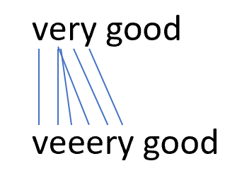
FIGURE 2.18: Time shift example between two sentences.

To compare two sequences we could use the well known Euclidean distance. However since the two sequences may not be aligned in time, the result could be misleading. Furthermore, the two sequences differ in length. To account for this “time-shift” effect in timeseries data, Dynamic Time Warping (DTW) (Sakoe et al. 1990) can be used instead. DTW is a method that:

Finds an optimal match between two time-dependent sequences.
Computes their dissimilarity.
Finds the optimal deformation (mapping) of one of the sequences onto the other.

Another advantage of DTW is that the timeseries do not need to be of the same length. Suppose we have two timeseries, a query, and a reference we want to compare with:

\[\begin{align*} query&=(2,2,2,4,4,3)\\ ref&=(2,2,3,3,2) \end{align*}\]

The first thing to note is that the sequences differ in length. Figure 2.19 shows their plot. The query is the solid line and seems to be shifted to the right one position with respect to the reference. The plot also shows the resulting alignment after applying the DTW algorithm (dashed lines between the sequences). The resulting distance (after aligning) between the sequences is $3$. In the following, we will see how the problem can be formalized and how it can be computed. Don’t worry if you find the math notation a bit difficult to grasp at this point. A step by step example will follow which should help to explain how the method works.

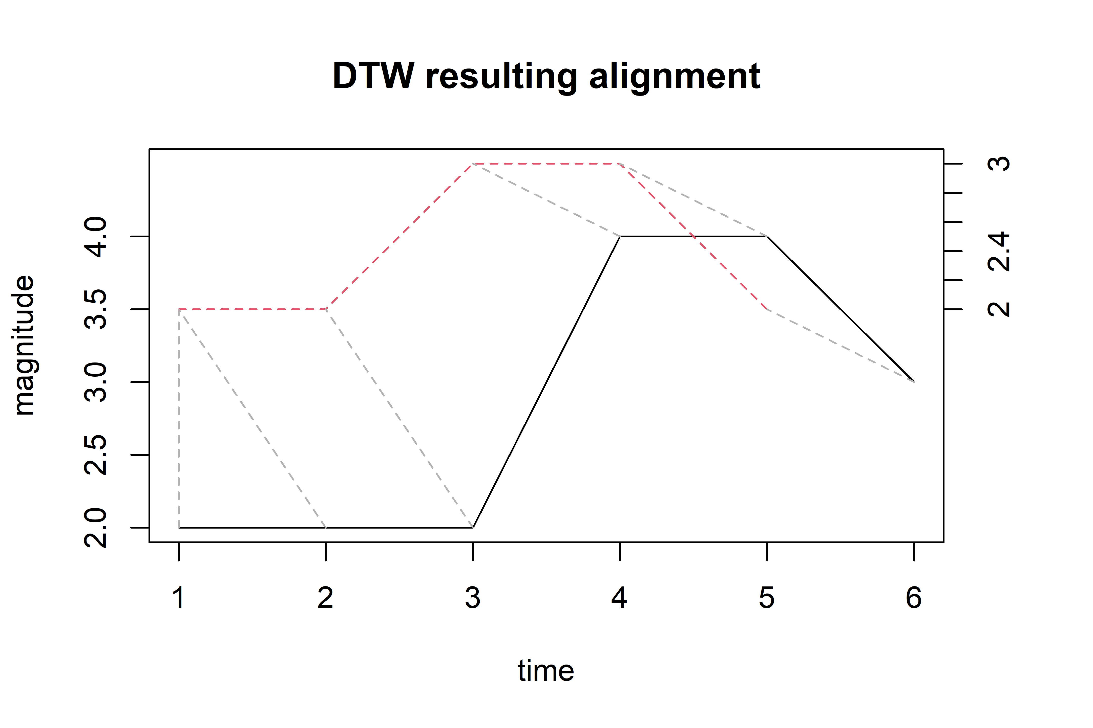
FIGURE 2.19: DTW alignment between the query and reference sequences (solid line is the query).

The problem of aligning two sequences can be formalized as follows (Rabiner and Juang 1993). Let $X$ and $Y$ be two sequences:

\[\begin{align*} X&=(x_1,x_2,\dots,x_{T_x}) \\ Y&=(y_1,y_2,\dots,y_{T_y}) \end{align*}\]

where $x_i$ and $y_i$ are vectors. In the previous example, the vectors only have one element since the sequences are $1$-dimensional, but DTW also works with multidimensional sequences. $T_x$ and $T_y$ are the sequences’ lengths. Let

\[\begin{align*} d(i_x,i_y) \end{align*}\]

be the dissimilarity (distance) between vectors $x_i$ and $y_i$ (e.g., Euclidean distance). Then, $\phi_x$ and $\phi_y$ are the warping functions that relate $i_x$ and $i_y$ to a common axis $k$:

\[\begin{align*} i_x&=\phi_x (k), k=1,2,\dots,T \\ i_y&=\phi_y (k), k=1,2,\dots,T. \end{align*}\]

The total dissimilarity between the two sequences is:

\[\begin{equation} d_\phi (X,Y) = \sum_{k=1}^T{d\left(\phi_x (k), \phi_y (k)\right)} \tag{2.14} \end{equation}\]

The aim is to find the warping function $\phi$ that minimizes the total dissimilarity:

\[\begin{equation} \operatorname*{min}_{\phi} d_\phi (X,Y) \tag{2.15} \end{equation}\]

The solution can be efficiently computed using dynamic programming. Usually, when solving this minimization problem, some constraints are applied:

Endpoint constraints. This constraint makes sure that the first and last elements of each sequence are connected (mapped to each other).

\[\begin{align*} \phi_x (1)&=1, \phi_y (1)=1 \\ \phi_x (T)&=T_x, \phi_y (T)=T_y \end{align*}\]

Monotonicity. This constraint allows ‘time to flow’ only from left to right. That is, we cannot go back in time.

\[\begin{align*} \phi_x (k+1) \geq \phi_x(k) \\ \phi_y (k+1) \geq \phi_y(k) \end{align*}\]

Local constraints. For example, allow jumps of at most $1$ step.

\[\begin{align*} \phi_x (k+1) - \phi_x(k) \leq 1 \\ \phi_y (k+1) - \phi_y(k) \leq 1 \end{align*}\]

Also, it is possible to apply global constraints, other local constraints, and apply different weights to slopes but the three described above are the most common ones. For a comprehensive list of constraints, please see (Rabiner and Juang 1993). Now let’s get back to our example and go through the steps to compute the dissimilarity and warping functions between our query ($Q$) and reference ($R$) sequences:

\[\begin{align*} Q&=(2,2,2,4,4,3) \\ R&=(2,2,3,3,2) \end{align*}\]

The first step is to compute a local cost matrix. This is just a matrix that contains the distance between every pair of points between the two sequences. For this example, we will use the Manhattan distance. Since our sequences are $1$-dimensional this distance can be computed as the absolute difference $|x_i - y_i|$. Figure 2.20 shows the resulting local cost matrix.

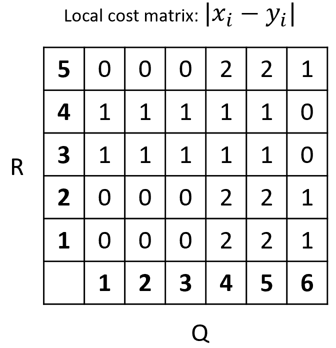
FIGURE 2.20: Local cost matrix between Q and R.

For example, position $(1,1)=0$ (row,column) because the first element of $Q$ is $2$ and the first element of $R$ is also $2$, thus, $|2-2|=0$. The rest of the matrix is filled in the same way. In dynamic programming, partial results are computed and stored in a table. Figure 2.21 shows the final dynamic programming table computed from the local cost matrix. Initially, this table is empty. We start to fill it from bottom left at position $(1,1)$. From the local cost matrix, the cost at position $(1,1)$ is $0$ so the cost at that position in the dynamic programming table is $0$. Then we can start filling in the contiguous cells. The only direction from which we can arrive at position $(1,2)$ is from the west (W). The cost at position $(1,2)$ from the local cost matrix is $0$ and the cost of the minimum of the cell from the west $(1,1)$ is also $0$. So $W:0+0=0$. For each cell we add the current cost plus the minimum cost when coming from the contiguous cell. The minimum costs are marked with red. For some cells it is possible to arrive from three different directions: S, W, and SW, thus we need to compute the cost when coming from each of those. The final minimum cost at position $(5,6)$ is $3$. Thus, that is the global DTW distance. In the example, it is possible to get the minimum at $(5,6)$ when arriving from the south or southwest.

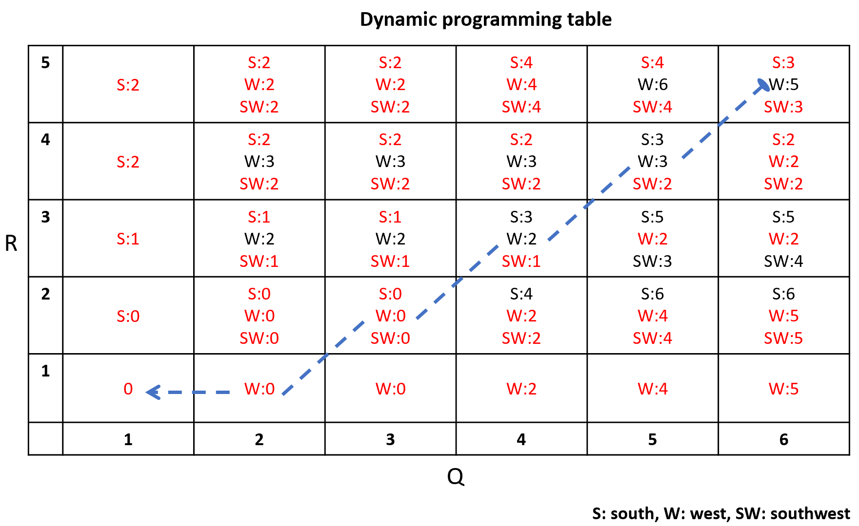
FIGURE 2.21: Dynamic programming table.

Once the table is filled in, we can backtrack starting at $(5,6)$ to find the warping functions. Figure 2.22 shows the final warping functions. Because of the endpoint constraints, we know that $\phi_Q(1)=1, \phi_R(1)=1$, $\phi_Q(6)=6$, and $\phi_R(6)=5$. Then, from $(5,6)$ the minimum contiguous value is $2$ coming from SW, thus $\phi_Q(5)=5, \phi_R(5)=4$, and so on. Note that we could also have chosen to arrive from the south with the same minimum value of $2$ but still this would have resulted in the same overall distance. The dashed line in figure 2.21 shows the full backtracking.

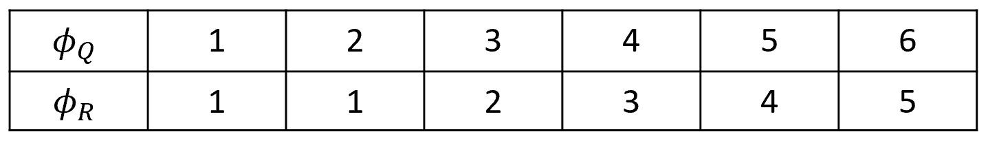
FIGURE 2.22: Resulting warping functions.

The runtime complexity of DTW is $O(T_x T_y)$. This is the required time to compute the local cost matrix and the dynamic programming table.

In R, the dtw package (Giorgino 2009) has the function dtw() to compute the DTW distance between two sequences. Let’s use this package to solve the previous example.

library("dtw")

# Sequences from the example
query <- c(2,2,2,4,4,3)
ref <- c(2,2,3,3,2)

# Find dtw distance.
alignment <- dtw(query, ref,
                 step = symmetric1, keep.internals = T)

The keep.internals = T keeps the input data so it can be accessed later, e.g., for plotting. The cost matrix and final distance can be accessed from the resulting object. The step argument specifies a step pattern. A step pattern describes some of the algorithm constraints such as endpoint and local constraints. In this case, we use symmetric1 which applies the constraints explained before. We can access the cost matrix, the final distance, and the warping functions $\phi_x$ and $\phi_y$ as follows:

alignment$localCostMatrix
#>      [,1] [,2] [,3] [,4] [,5]
#> [1,]    0    0    1    1    0
#> [2,]    0    0    1    1    0
#> [3,]    0    0    1    1    0
#> [4,]    2    2    1    1    2
#> [5,]    2    2    1    1    2
#> [6,]    1    1    0    0    1

alignment$distance
#> [1] 3

alignment$index1
#> [1] 1 2 3 4 5 6

alignment$index2
#> [1] 1 1 2 3 4 5

The local cost matrix is the same one as in Figure 2.20 but in rotated form. The resulting object also has the dynamic programming table which can be plotted along with the resulting backtracking (see Figure 2.23).

ccm <- alignment$costMatrix
image(x = 1:nrow(ccm), y = 1:ncol(ccm),
      ccm, xlab = "Q", ylab = "R")
text(row(ccm), col(ccm), label = ccm)
lines(alignment$index1, alignment$index2)

FIGURE 2.23: Dynamic programming table and backtracking.

And finally, the aligned sequences can be plotted. The previous Figure 2.19 shows the result of the following command.

plot(alignment, type="two", off=1.5,
     match.lty=2,
     match.indices=10,
     main="DTW resulting alignment",
     xlab="time", ylab="magnitude")

2.5.1 Hand Gesture Recognition

hand_gestures.R, hand_gestures_auxiliary.R

Gestures are a form of communication. They are often accompanied with speech but can also be used to communicate something independently of speech (like in sign language). Gestures allow us to externalize and emphasize emotions and thoughts. They are based on body movements from arms, hands, fingers, face, head, etc. Gestures can be used as a non-verbal way to identify and study behaviors for different purposes such as for emotion (De Gelder 2006) or for the identification of developmental disorders like autism (Anzulewicz, Sobota, and Delafield-Butt 2016).

Gestures can also be used to develop user-computer interaction applications. The following video shows an example application of gesture recognition for domotics.

The application determines the indoor location using $k$-NN as it was shown in this chapter. The gestures are classified using DTW (I’ll show how to do it in a moment). Based on the location and type of gesture, an specific home appliance is activated. I programmed that app some time ago using the same algorithms presented here.

To demonstrate how DTW can be used for hand gesture recognition, we will examine the HAND GESTURES dataset that was collected with a smartphone using its accelerometer sensor. The data was collected by $10$ individuals who performed $5$ repetitions of $10$ different gestures (‘triangle’, ‘square’, ‘circle’, ‘a’, ‘b’, ‘c’, ‘1’, ‘2’, ‘3’, ‘4’). The sensor is a tri-axial accelerometer that returns values for the $x$, $y$, and $z$ axes. The participants were not instructed to hold the smartphone in any particular way. The sampling rate was set at $50$ Hz. To record a gesture, the user presses the phone’s screen with her/his thumb, performs the gesture in the air, and stops pressing the screen after the gesture is complete. Figure 2.24 shows the start and end positions of the $10$ gestures.

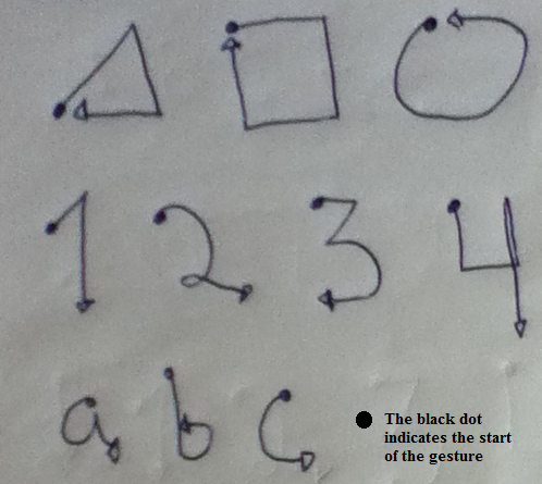
FIGURE 2.24: Paths for the 10 considered gestures.

In order to make the recognition orientation-independent, we can compute the magnitude of the $3$ accelerometer axes. This will provide us with the overall movement patterns regardless of orientation.

\[\begin{equation} Magnitude(t) = \sqrt {{a_x}{{(t)}^2} + {a_y}{{(t)}^2} + {a_z}{{(t)}^2}} \tag{2.16} \end{equation}\]

where ${a_x}{{(t)}}$, ${a_y}{{(t)}}$, and ${a_z}{{(t)}}$ are the accelerations at time $t$.

Figure 2.25 shows the raw accelerometer values (dashed lines) for a triangle gesture. The solid line shows the resulting magnitude. This will also simplify things since we will now work with $1$-dimensional sequences (the magnitudes) instead of the other $3$ axes.

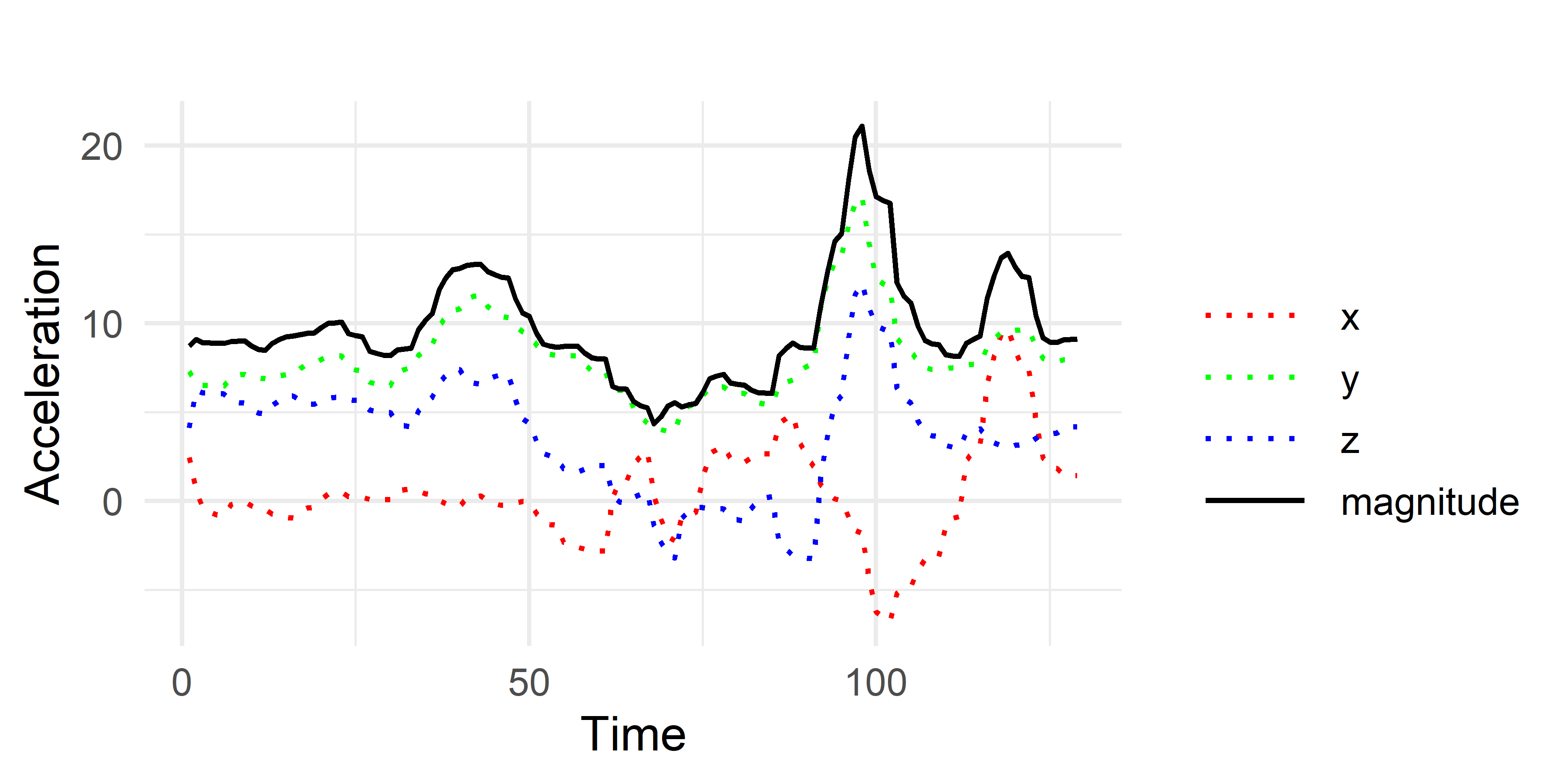
FIGURE 2.25: Triangle gesture.

The gestures are stored in text files that contain the $x$, $y$, and $z$ recordings. The script hand_gestures_auxiliary.R has some auxiliary functions to preprocess the data. Since the sequences of each gesture are of varying length, storing them as a data frame could be problematic because data frames have fixed sizes. Instead, the gen.instances() function processes the files and returns all hand gestures as a list. This function also computes the magnitude (equation (2.16)). The following code (from hand_gestures.R) calls the gen.instances() function and stores the results in the instances variable which is a list. Then, we select the first and second instances to be the query and the reference.

# Format instances from files.
instances <- gen.instances("../data/hand_gestures/")

# Use first instance as the query.
query <- instances[[1]]

# Use second instance as the reference.
ref <- instances[[2]]

Each element in instances is also a list that stores the type and values (magnitude) of each gesture.

# Print their respective classes
print(query$type)
#> [1] "1"

print(ref$type)
#> [1] "1"

Here, the first two instances are of type ‘1’. We can also print the magnitude values.

# Print values.
print(query$values)
#> [1]  9.167477  9.291464  9.729926  9.901090  ....

In this case, both classes are “1”. We can use the dtw() function to compute the similarity between the query and the reference instance and plot the resulting alignment (Figure 2.26).

alignment <- dtw(query$values, ref$values, keep = TRUE)

# Print similarity (distance)
alignment$distance
#> [1] 68.56493

# Plot result.
plot(alignment, type="two", off=1, match.lty=2, match.indices=40,
     main="DTW resulting alignment",
     xlab="time", ylab="magnitude")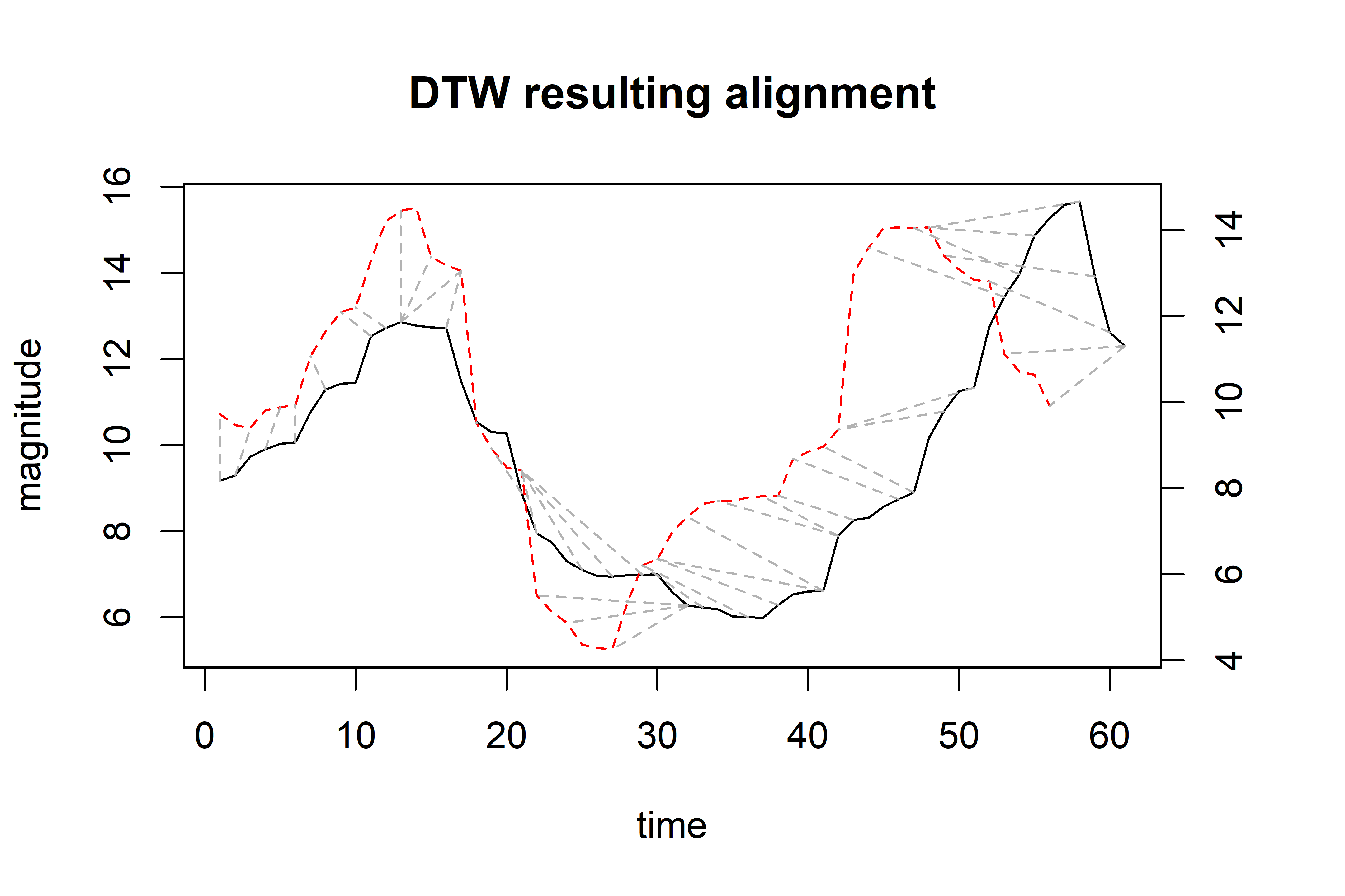

FIGURE 2.26: Resulting alignment.

To perform the actual classification, we will use our well-known $k$-NN classifier with $k=1$. To classify a query instance, we need to compute its DTW distance to every other instance in the training set and predict the label from the closest one. We will test the performance using $10$-fold cross-validation. Since computing all DTW distances takes some time, we can precompute all pairs of distances and store them in a matrix. The auxiliary function matrix.distances() does the job. Since this can take some minutes, the results are saved so there is no need to wait next time the code is run.

D <- matrix.distances(instances)

# Save results.
save(D, file="D.RData")

The matrix.distances() returns a list. The first element is an array with the gestures’ classes and the second element is the actual distance matrix. The elements in the diagonal are set to Inf to signal that we don’t want to take into account the dissimilarity between a gesture and itself.

For convenience, this matrix is already stored in the file D.RData located this chapter’s code directory. The following code performs the $10$-fold cross-validation and computes the performance results.

# Load the DTW distances matrix.
load("D.RData")
set.seed(1234)
k <- 10 # Number of folds.
folds <- sample(k, size = length(D[[1]]), replace = T)
predictions <- NULL
groundTruth <- NULL

# Implement k-NN with k=1.
for(i in 1:k){
  
  trainSet <- which(folds != i)
  testSet <- which(folds == i)
  train.labels <- D[[1]][trainSet]
  
  for(query in testSet){
    
    type <- D[[1]][query]
    distances <- D[[2]][query, ][trainSet]
    
    # Return the closest one.
    nn <- sort(distances, index.return = T)$ix[1]
    pred <- train.labels[nn]
    predictions <- c(predictions, pred)
    groundTruth <- c(groundTruth, type)
    
  }
} # end of for

The line distances <- D[[2]][query, ][trainSet] retrieves the pre-computed distances between the test query and all gestures in the train set. Then, those distances are sorted in ascending order and the class of the closest one is used as the prediction. Finally, the performance is calculated.

cm <- confusionMatrix(factor(predictions),
                      factor(groundTruth))

# Compute performance metrics per class.
cm$byClass[,c("Recall", "Specificity", "Precision", "F1")]
#>                   Recall Specificity Precision        F1
#> Class: 1            0.84   0.9911111 0.9130435 0.8750000
#> Class: 2            0.84   0.9866667 0.8750000 0.8571429
#> Class: 3            0.96   0.9911111 0.9230769 0.9411765
#> Class: 4            0.98   0.9933333 0.9423077 0.9607843
#> Class: a            0.78   0.9733333 0.7647059 0.7722772
#> Class: b            0.76   0.9955556 0.9500000 0.8444444
#> Class: c            0.90   1.0000000 1.0000000 0.9473684
#> Class: circleLeft   0.78   0.9622222 0.6964286 0.7358491
#> Class: square       1.00   0.9977778 0.9803922 0.9900990
#> Class: triangle     0.92   0.9711111 0.7796610 0.8440367

# Overall performance metrics
colMeans(cm$byClass[,c("Recall", "Specificity",
                       "Precision", "F1")])
#>     Recall Specificity   Precision          F1 
#>  0.8760000   0.9862222   0.8824616   0.8768178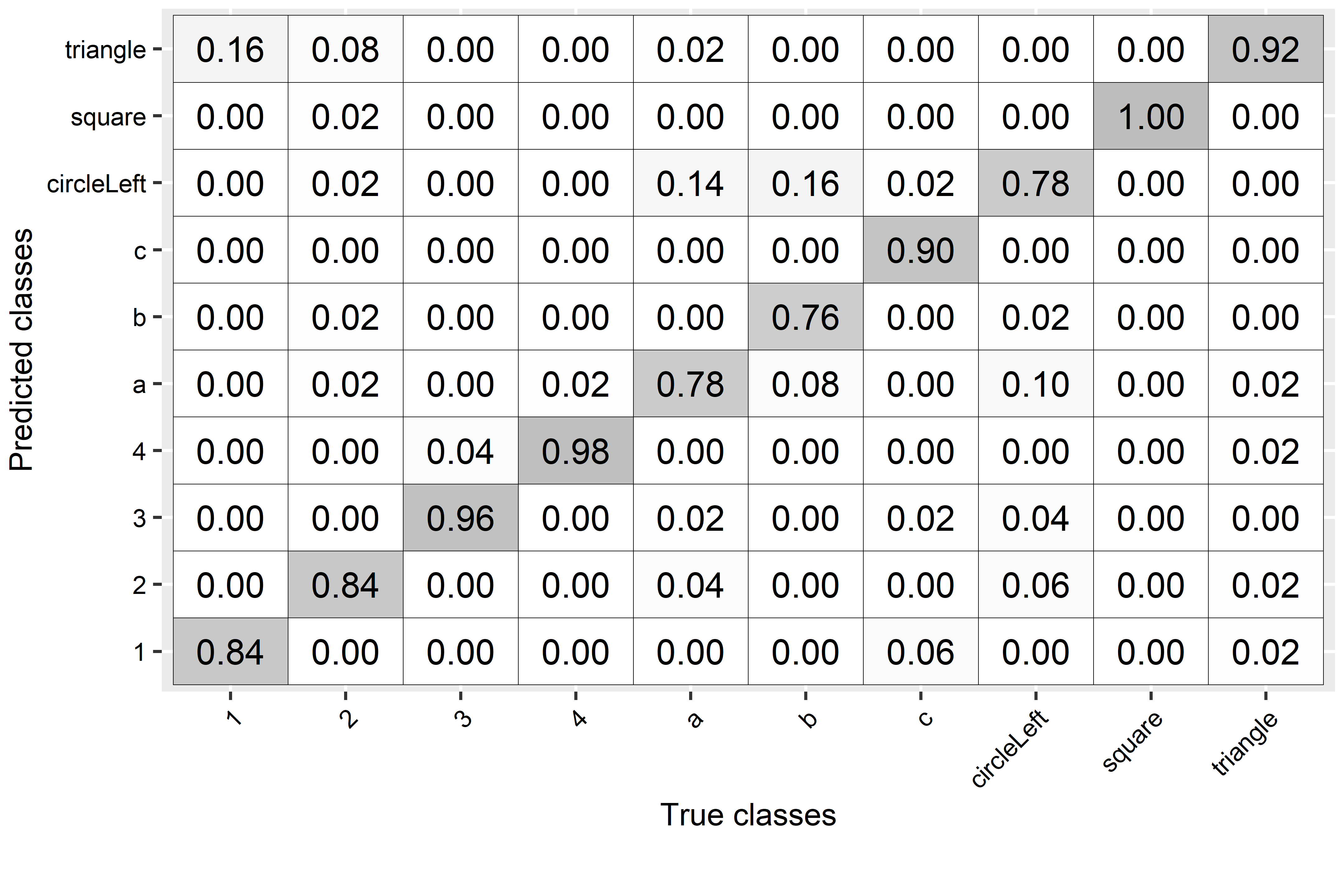

FIGURE 2.27: Confusion matrix for hand gestures’ predictions.

The overall recall was $0.87$ which is not bad. From the confusion matrix (Figure 2.27), we can see that the class ‘a’ was often confused with ‘circleLeft’ and vice versa. This makes sense since both have similar motions (see Figure 2.24). Also, ‘b’ was often confused with ‘circleLeft’. The ‘square’ class was always correctly classified. This example demonstrated how DTW can be used with $k$-NN to recognize hand gestures.

2.6 Dummy Models

dummy_classifiers.R

When faced with a new problem, you may be tempted to start trying to solve it by using a complex model. Then, you proceed to train your complex model and evaluate it. The results look reasonably good so you think you are done. However, this good performance could only be an illusion. Sometimes there are underlying problems with the data that can give the false impression that a model is performing well. Examples of such problems are imbalanced datasets, no correlation between the features and the classes, features not containing enough information, etc. Dummy models can be used to spot some of those problems. Dummy models use little or no information at all when making predictions (we’ll see how in a moment).

Furthermore, for some problems (specially in regression) it is not clear what is considered to be a good performance. There are problems in which doing slightly better than random is considered a great achievement (e.g., in forecasting) but for other problems that would be unacceptable. Thus, we need some type of baseline to assess whether or not a particular model is bringing some benefit. Dummy models are not only used to spot problems but can be used as baselines as well.

Dummy models are also called baseline models or dumb models. One student I was supervising used to call them stupid models. When I am angry, I also call them like that, but today I’m in a good mood so I’ll refer to them as dummy.

Now, I will present three types of dummy classifiers and how they can be implemented in R.

2.6.1 Most-frequent-class Classifier

As the name implies, the most-frequent-class classifier always predicts the most frequent label found in the train set. This means that the model does not even need to look at the features! Once it is presented with a new instance, it just outputs the most common class as the prediction.

To show how it can be implemented, I will use the SMARTPHONES ACTIVITIES dataset. For demonstration purposes, I will only keep two classes: ‘Walking’ and ‘Upstairs’. Furthermore, I will only pick a small percent of the instances with class ‘Upstairs’ to simulate an imbalanced dataset. Imbalanced means that there are classes for which only a few instances exist. More about imbalanced data and how to handle it will be covered in chapter 5. After those modifications, we can check the class counts:

# Print class counts.
table(dataset$class)
#> Upstairs  Walking 
#>      200     2081

# In percentages.
table(dataset$class) / nrow(dataset)
#>   Upstairs    Walking 
#> 0.08768084 0.91231916

We can see that more than $90\%$ of the instances belong to class ‘Walking’. It’s time to define the dummy classifier!

# Define the dummy classifier's train function.
most.frequent.class.train <- function(data){
  
  # Get a table with the class counts.
  counts <- table(data$class)
  
  # Select the label with the most counts.
  most.frequent <- names(which.max(counts))
  
  return(most.frequent)
}

The most.frequent.class.train() function will learn the parameters from a train set. The only thing this model needs to learn is what is the most frequent class. First, the table() function is used to get the class counts and then the name of the class with the max counts is returned. Now we define the predict function which takes as its first argument the learned parameters and as second argument the test set on which we want to make predictions. The parameter only consists of the name of a class.

# Define the dummy classifier's predict function.
most.frequent.class.predict <- function(params, data){

  # Return the same label for as many rows as there are in data.
  return(rep(params, nrow(data)))
  
}

The only thing the predict function does is to return the params argument that contains the class name repeated $n$ times. Where $n$ is the number of rows in the test data frame.

Let’s try our functions. The dataset has already been split into $50\%$ for training and $50\%$ for testing. First we train the dummy model using the train set. Then, the learned parameter is printed.

# Learn the parameters.
dummy.model1 <- most.frequent.class.train(trainset)

# Print the learned parameter.
dummy.model1
#> [1] "Walking"

Now we can make predictions on the test set and compute the accuracy.

# Make predictions.
predictions <- most.frequent.class.predict(dummy.model1, testset)

# Compute confusion matrix and other performance metrics.
cm <- confusionMatrix(factor(predictions, levels),
                       factor(testset$class, levels))

# Print accuracy
cm$overall["Accuracy"]
#>  Accuracy 
#>  0.9087719

The accuracy was $90.8\%$. It seems that the dummy classifier was not that dummy after all! Let’s print the confusion matrix to inspect the predictions.

# Print confusion matrix.
cm$table

#>           Reference
#> Prediction Walking Upstairs
#>   Walking     1036      104
#>   Upstairs       0        0

From the confusion matrix we can see that all ‘Walking’ activities were correctly classified but none of the ‘Upstairs’ classes were identified. This is because the dummy model only predicts ‘Walking’. Here we can see that even though it seemed like the dummy model was doing pretty good, it was not that good after all.

We can now try with a decision tree from the rpart package.

### Let's try with a decision tree
treeClassifier <- rpart(class ~ ., trainset)

tree.predictions <- predict(treeClassifier, testset, type = "class")

cm.tree <- confusionMatrix(factor(tree.predictions, levels),
                      factor(testset$class, levels))

# Print accuracy
cm.tree$overall["Accuracy"]
#>  Accuracy 
#> 0.9263158

Decision trees are more powerful than dummy classifiers but the accuracy was very similar!

It is a good practice to compare powerful models against dummy models. If their performances are similar, this may be an indication that there is something that needs to be checked. In this example, the problem was that the dataset was imbalanced. It is also adivisable to report not only the accuracy but other metrics. We could also have noted the imbalance problem by looking at the recall of the individual classes, for example.

2.6.2 Uniform Classifier

This is another type of dummy classifier. This one predicts classes at random with equal probability and can be implemented as follows.

# Define the dummy classifier's train function.
uniform.train <- function(data){
  
  # Get the unique classes.
  unique.classes <- unique(data$class)
  
  return(unique.classes)
}

# Define the dummy classifier's predict function.
uniform.predict <- function(params, data){
  
  # Sample classes uniformly.
  return(sample(unique.classes, size = nrow(data), replace = T))
  
}

At prediction time, it just picks a random label for each instance in the test set. This model achieved an accuracy of only $49.0\%$ using the same dataset, but it correctly identified more classes of type ‘Upstairs’.

#>           Reference
#> Prediction Walking Upstairs
#>   Walking      506       54
#>   Upstairs     530       50

If a dataset is balanced and the accuracy of the uniform classifier is similar to the more complex model, the problem may be that the features are not providing enough information. That is, the complex classifier was not able to extract any useful patterns from the features.

2.6.3 Frequency-based Classifier

This one is similar to the uniform classifier but the probability of choosing a class is proportional to its frequency in the train set. Its implementation is similar to the uniform classifier but makes use of the prob parameter in the sample() function to specify weights for each class. The higher the weight for a class, the more probable it will be chosen at prediction time. The implementation of this one is in the script dummy_classifiers.R.

The frequency-based classifier achieved an accuracy of $85.5\%$. Much lower than the most-frequent-class model ($90.8\%$) but it was able to detect some of the ‘Upstairs’ classes.

2.6.4 Other Dummy Classifiers

Another dummy model that can be used for classification is to apply simple thresholds.

if(feature1 < threshold)
  return("A")
else
  return("B")

In fact, the previous rule can be thought of as a very simple decision tree with only one root node. Surprisingly, sometimes simple rules can be difficult to beat by more complex models. In this section I’ve been focusing on classification problems, but dummy models can also be constructed for regression. The simplest one would be to predict the mean value of $y$ regardless of the feature values. Another dummy model could predict a random value between the min and max of $y$. If there is a categorical feature, one could predict the mean value based on the category. In fact, that is what we did in chapter 1 in the simple regression example.

In summary, one can construct any type of dummy model depending on the application. The takeaway is that dummy models allow us to assess how more complex models perform with respect to some baselines and help us to detect possible problems in the data and features. What I typically do when solving a problem is to start with simple models and/or rules and then, try more complex models. Of course, manual thresholds and simple rules can work remarkably well in some situations but they are not scalable. Depending on the use case, one can just implement the simple solution or go for something more complex if the system is expected to grow or be used in more general ways.

2.7 Summary

This chapter focused on classification models. Classifiers predict a category based on the input features. Here, it was demonstrated how classifiers can be used to detect indoor locations, classify activities, and hand gestures.

$k$-Nearest Neighbors ($k$-NN) predicts the class of a test point as the majority class of the $k$ nearest neighbors.
Some classification performance metrics are recall, specificity, precision, accuracy, F1-score, etc.
Decision trees are easy-to-interpret classifiers trained recursively based on feature importance (for example, purity).
Naive Bayes is a type of classifier where features are assumed to be independent.
Dynamic Time Warping (DTW) computes the similarity between two timeseries after aligning them in time. This can be used for classification for example, in combination with $k$-NN.
Dummy models can help to spot possible errors in the data and can also be used as baselines.

References

Anzulewicz, Anna, Krzysztof Sobota, and Jonathan T Delafield-Butt. 2016. “Toward the Autism Motor Signature: Gesture Patterns During Smart Tablet Gameplay Identify Children with Autism.” Scientific Reports 6 (1): 1–13.

De Gelder, Beatrice. 2006. “Towards the Neurobiology of Emotional Body Language.” Nature Reviews Neuroscience 7 (3): 242–49.

Giorgino, Toni. 2009. “Computing and Visualizing Dynamic Time Warping Alignments in r: The dtw Package.” Journal of Statistical Software 31 (7): 1–24.

Kwapisz, Jennifer R., Gary M. Weiss, and Samuel A. Moore. 2010. “Activity Recognition Using Cell Phone Accelerometers.” In Proceedings of the Fourth International Workshop on Knowledge Discovery from Sensor Data (at KDD-10), Washington DC.

Meyer, David, Evgenia Dimitriadou, Kurt Hornik, Andreas Weingessel, and Friedrich Leisch. 2019. E1071: Misc Functions of the Department of Statistics, Probability Theory Group (Formerly: E1071), TU Wien. https://CRAN.R-project.org/package=e1071.

Milborrow, Stephen. 2019. Rpart.plot: Plot “Rpart” Models: An Enhanced Version of “plot.rpart”. https://CRAN.R-project.org/package=rpart.plot.

Quinlan, J Ross. 2014. C4.5: Programs for Machine Learning. San Mateo, California: Morgan Kaufmann Publishers.

Rabiner, Lawrence, and Biing-Hwang Juang. 1993. Fundamentals of Speech Recognition. Englewood Cliffs, New Jersey: Prentice hall.

Sakoe, Hiroaki, Seibi Chiba, A Waibel, and KF Lee. 1990. “Dynamic Programming Algorithm Optimization for Spoken Word Recognition.” Readings in Speech Recognition 159: 224.

Steinberg, Dan, and Phillip Colla. 2009. “CART: Classification and Regression Trees.” The Top Ten Algorithms in Data Mining 9: 179.

Therneau, Terry, and Beth Atkinson. 2019. Rpart: Recursive Partitioning and Regression Trees. https://CRAN.R-project.org/package=rpart.

Xi, Xiaopeng, Eamonn Keogh, Christian Shelton, Li Wei, and Chotirat Ann Ratanamahatana. 2006. “Fast Time Series Classification Using Numerosity Reduction.” In Proceedings of the 23rd International Conference on Machine Learning, 1033–40.