Chapter 3 Predicting Behavior with Ensemble Learning
In the previous chapters, we have been building single models, either for classification or regression. With ensemble learning, the idea is to train several models and combine their results to increase the performance. Usually, ensemble methods outperform single models. In the context of ensemble learning, the individual models whose results are to be combined are known as base learners. Base learners can be of the same type (homogeneous) or of different types (heterogeneous). Examples of ensemble methods are Bagging, Random Forest, and Stacked Generalization. In the following sections, the three of them will be described and example applications in behavior analysis will be presented as well.
3.1 Bagging
Bagging stands for “bootstrap aggregating” and is an ensemble learning method proposed by Breiman (1996). Ummm…, Bootstrap, aggregating? Let’s start with the aggregating part. As the name implies, this method is based on training several base learners (e.g., decision trees) and combining their outputs to produce a single final prediction. One way to combine the results is by taking the majority vote for classification tasks or the average for regression. In an ideal case, we would have enough data to train each base learner with an independent train set. However, in practice we may only have a single train set of limited size. Training several base learners with the same train set is equivalent to having a single learner, provided that the training procedure of the base learners is deterministic. Even if the training procedure is not deterministic, the resulting models might be very similar. What we would like to have is accurate base learners but at the same time they should be diverse. Then, how can those base learners be trained? Well, this is where the bootstrap part comes into play.
Bootstrapping means generating new train sets by sampling instances with replacement from the original train set. If the original train set has \(N\) instances, the method selects \(N\) instances at random to produce a new train set. With replacement means that repeated instances are allowed. This has the effect of generating a new train set of size \(N\) by removing some instances and duplicating other instances. By using this method, \(n\) different train sets can be generated and used to train \(n\) different learners.
It has been shown that having more diverse base learners increases performance. One way to generate diverse learners is by using different train sets as just described. In his original work, Breiman (1996) used decision trees as base learners. Decision trees are considered to be very unstable. This means that small changes in the train set produce very different trees - but this is a good thing for bagging! Most of the time, the aggregated predictions will produce better results than the best individual learner from the ensemble.
Figure 3.1 shows bootstrapping in action. The train set is sampled with replacement \(3\) times. The numbers represent indices to arbitrary train instances. Here, we can see that in the first sample, the instance number \(5\) is missing but instead, instance \(2\) is duplicated. All samples have five elements. Then, each sample is used to train individual decision trees.
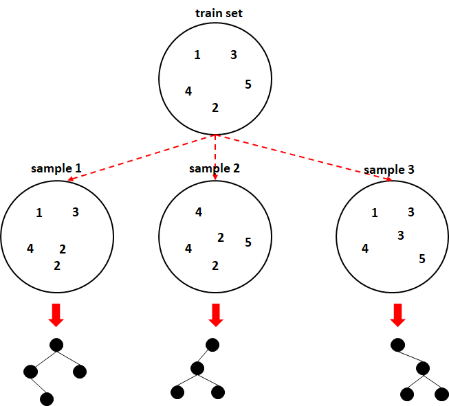
FIGURE 3.1: Bagging example.
One of the disadvantages of ensemble methods is their higher computational cost both during training and inference. Another disadvantage of ensemble methods is that they are more difficult to interpret. Still, there exist model agnostic interpretability methods (Molnar 2019) that can help to analyze the results. In the next section, I will show you how to implement your own Bagging model with decision trees in R.
3.1.1 Activity Recognition with Bagging
bagging_activities.R iterated_bagging_activities.R
In this section, we will implement Bagging with decision trees. Then, we will test our implementation on the SMARTPHONE ACTIVITIES dataset. The following code snippet shows the implementation of the my_bagging() function. The complete code is in the script bagging_activities.R. The function accepts three arguments. The first one is the formula, the second one is the train set, and the third argument is the number of base learners (\(10\) by default). Here, we will use the rpart package to train the decision trees.
# Define our bagging classifier.
my_bagging <- function(theFormula, data, ntrees = 10){

  N <- nrow(data)

  # A list to store the individual trees
  models <- list()

  # Train individual trees and add each to 'models' list.
  for(i in 1:ntrees){

    # Bootstrap instances from data.
    idxs <- sample(1:N, size = N, replace = T)

    bootstrappedInstances <- data[idxs,]

    treeModel <- rpart(as.formula(theFormula),
                       bootstrappedInstances,
                       xval = 0,
                       cp = 0)

    models <- c(models, list(treeModel))
  }

  res <- structure(list(models = models),
                   class = "my_bagging")

  return(res)
}
First, a list that will store each individual learner is defined models <- list(). Then, the function iterates ntrees times. In each iteration, a bootstrapped train set is generated and used to train a rpart model. The xval = 0 parameter tells rpart not to perform cross-validation internally. The cp parameter is also set to \(0\). This value controls the amount of pruning. The default is \(0.01\) leading to smaller trees. This makes the trees to be more similar but since we want diversity we are setting this to \(0\) so bigger trees are generated and as a consequence, more diverse.
Finally, an object of class "my_bagging" is returned. This is just a list containing the trained base learners. The class = "my_bagging" argument is important. It tells R that this object is of type my_bagging. Setting the class will allow us to use the generic predict() function, and R will automatically call the corresponding predict.my_bagging() function which we will shortly define. The class name and the function name after predict. need to be the same.
# Define the predict function for my_bagging.
predict.my_bagging <- function(object, newdata){

  ntrees <- length(object$models)
  N <- nrow(newdata)

  # Matrix to store predictions for each instance
  # in newdata and for each tree.
  M <- matrix(data = rep("",N * ntrees), nrow = N)

  # Populate matrix.
  # Each column of M contains all predictions for a given tree.
  # Each row contains the predictions for a given instance.
  for(i in 1:ntrees){
    m <- object$models[[i]]
    tmp <- as.character(predict(m, newdata, type = "class"))
    M[,i] <- tmp
  }

  # Final predictions
  predictions <- character()

  # Iterate through each row of M.
  for(i in 1:N){
    # Compute class counts
    classCounts <- table(M[i,])

    # Get the class with the most counts.
    predictions <- c(predictions,
                     names(classCounts)[which.max(classCounts)])
  }
  return(predictions)
}
Now let’s dissect the predict.my_bagging() function. First, note that the function name starts with predict. followed by the type of object. Following this convention will allow us to call predict() and R will call the corresponding method based on the class of the object. The first argument object is an object of type “my_bagging” as returned by my_bagging(). The second argument newdata is the test set we want to generate predictions for. A matrix M that will store the predictions for each tree is defined. This matrix has \(N\) rows and \(ntrees\) columns where \(N\) is the number of instances in newdata and \(ntrees\) is the number of trees. Thus, each column stores the predictions for each of the base learners. This function iterates through each base learner (rpart in this case), and makes a prediction for each instance in newdata. Then, the results are stored in matrix M. Finally, it iterates through each instance and computes the most common predicted class from the base learners.
Let’s test our Bagging function! We will test it with the activity recognition dataset introduced in section 2.3.1 and set the number of trees to \(10\). The following code shows how to use our bagging functions to train the model and make predictions on a test set.
baggingClassifier <- my_bagging(class ~ ., trainSet, ntree = 10)
predictions <- predict(baggingClassifier, testSet)
The following will perform \(5\)-fold cross-validation and print the results.
set.seed(1234)
k <- 5
folds <- sample(k, size = nrow(df), replace = TRUE)

# Variable to store ground truth classes.
groundTruth <- NULL

# Variable to store the classifier's predictions.
predictions <- NULL

for(i in 1:k){
  trainSet <- df[which(folds != i), ]
  testSet <- df[which(folds == i), ]
  treeClassifier <- my_bagging(class ~ ., trainSet, ntree = 10)
  foldPredictions <- predict(treeClassifier, testSet)
  predictions <- c(predictions, as.character(foldPredictions))
  groundTruth <- c(groundTruth, as.character(testSet$class))
}
cm <- confusionMatrix(as.factor(predictions), as.factor(groundTruth))

# Print accuracy
cm$overall["Accuracy"]
#> Accuracy
#> 0.861388

# Print other metrics per class.
cm$byClass[,c("Recall", "Specificity", "Precision", "F1")]
#>                      Recall Specificity Precision        F1
#> Class: Downstairs 0.5378788   0.9588957 0.5855670 0.5607108
#> Class: Jogging    0.9618462   0.9820722 0.9583078 0.9600737
#> Class: Sitting    0.9607843   0.9982394 0.9702970 0.9655172
#> Class: Standing   0.9146341   0.9988399 0.9740260 0.9433962
#> Class: Upstairs   0.5664557   0.9563310 0.6313933 0.5971643
#> Class: Walking    0.9336857   0.9226850 0.8827806 0.9075199

# Print average performance metrics across classes.
colMeans(cm$byClass[,c("Recall", "Specificity", "Precision", "F1")])
#>     Recall Specificity   Precision          F1
#>  0.8125475   0.9695105   0.8337286   0.8223970
The accuracy was much better now compared to \(0.789\) from the previous chapter without using Bagging!
The effect of adding more trees to the ensemble can also be analyzed. The script iterated_bagging_activities.R does \(5\)-fold cross-validation as we just did but starts with \(1\) tree in the ensemble and repeats the process by adding more trees until \(50\).
Figure 3.2 shows the effect on the train and test accuracy with different number of trees. Here, we can see that \(3\) trees already produce a significant performance increase compared to \(1\) or \(2\) trees. This makes sense since having only \(2\) trees does not add additional information. If the two trees produce different predictions then, it becomes a random choice between the two labels. In fact, \(2\) trees produced worse results than \(1\) tree. But we cannot make strong conclusions since the experiment was run only once. One possibility to break ties when there are only two trees is to use the averaged probabilities of each label. rpart can return those probabilities by setting type = "prob" in the predict() function which is the default behavior. This is left as an exercise for the reader. In the following section, Random Forest will be described which is a way of introducing more diversity to the base learners.
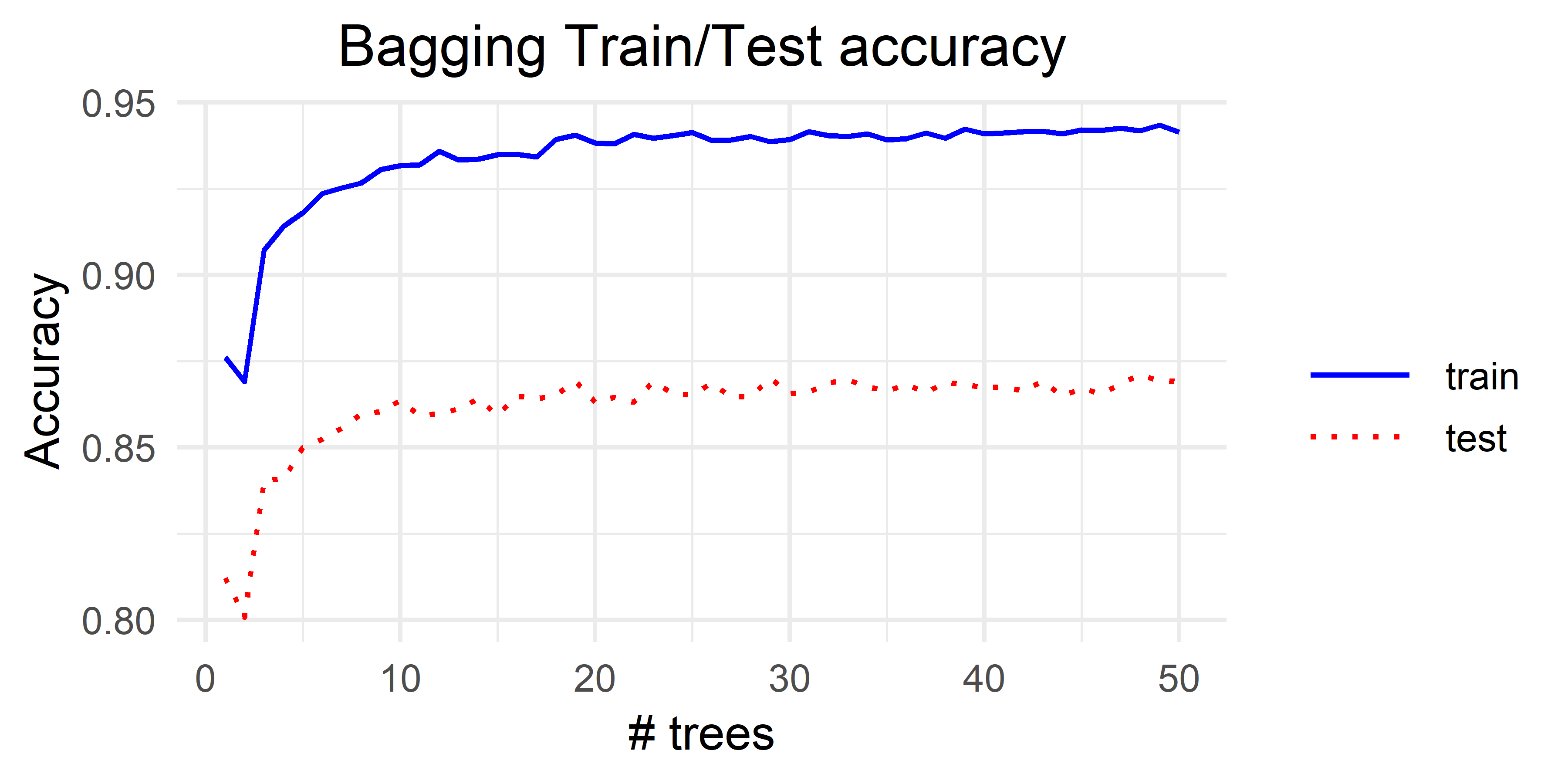
FIGURE 3.2: Bagging results for different number of trees.
3.2 Random Forest
rf_activities.R iterated_rf_activities.R iterated_bagging_rf.R
A Random Forest can be thought of as an extension of Bagging. Random Forests were proposed by Breiman (2001) and as the name implies, they introduce more randomness to the individual trees. This is with the objective of having decorrelated trees. With Bagging, most of the trees are very similar at the root because the most important variables are selected first (see chapter 2). To avoid this happening, a simple modification can be introduced. When building a tree, instead of evaluating all features at each split to find the most important one (based on some purity measure like information gain), a random subset of the features (usually \(\sqrt{|features|}\)) is sampled. This simple modification produces more decorrelated trees and in general, it results in better performance compared to Bagging.
In R, the most famous library that implements Random Forest is…, yes you guessed it: randomForest (Liaw and Wiener 2002). The following code snippet shows how to fit a Random Forest with \(10\) trees.
By default, ntree = 500. Among other things, you can control how many random features are sampled at each split with the mtry argument. By default, for classification mtry = floor(sqrt(ncol(x))) and for regression mtry = max(floor(ncol(x)/3), 1).
The following code performs \(5\)-fold cross-validation with the activities dataset already stored in df and prints the results. The complete code can be found in the script randomForest_activities.R.
set.seed(1234)

k <- 5

folds <- sample(k, size = nrow(df), replace = TRUE)

# Variable to store ground truth classes.
groundTruth <- NULL

# Variable to store the classifier's predictions.
predictions <- NULL

for(i in 1:k){

  trainSet <- df[which(folds != i), ]
  testSet <- df[which(folds == i), ]

  rf <- randomForest(class ~ ., trainSet, ntree = 10)

  foldPredictions <- predict(rf, testSet)

  predictions <- c(predictions, as.character(foldPredictions))

  groundTruth <- c(groundTruth, as.character(testSet$class))
}

cm <- confusionMatrix(as.factor(predictions), as.factor(groundTruth))

# Print accuracy
cm$overall["Accuracy"]
#>Accuracy
#> 0.870801

# Print other metrics per class.
cm$byClass[,c("Recall", "Specificity", "Precision", "F1")]
#>                      Recall Specificity Precision        F1
#> Class: Downstairs 0.5094697   0.9652352 0.6127563 0.5563599
#> Class: Jogging    0.9784615   0.9831268 0.9613059 0.9698079
#> Class: Sitting    0.9803922   0.9992175 0.9868421 0.9836066
#> Class: Standing   0.9512195   0.9990333 0.9790795 0.9649485
#> Class: Upstairs   0.5363924   0.9636440 0.6608187 0.5921397
#> Class: Walking    0.9543489   0.9151933 0.8752755 0.9131034

# Print other metrics overall.
colMeans(cm$byClass[,c("Recall", "Specificity", "Precision", "F1")])
#>     Recall Specificity   Precision          F1
#>  0.8183807   0.9709083   0.8460130   0.8299943
Those results are better than the previous ones with Bagging. Figure 3.3 shows the results when doing \(5\)-fold cross-validation for different number of trees (the complete script is in iterated_randomForest_activities.R). From these results, we can see a similar behavior as Bagging. That is, the accuracy increases very quickly and then it stabilizes.
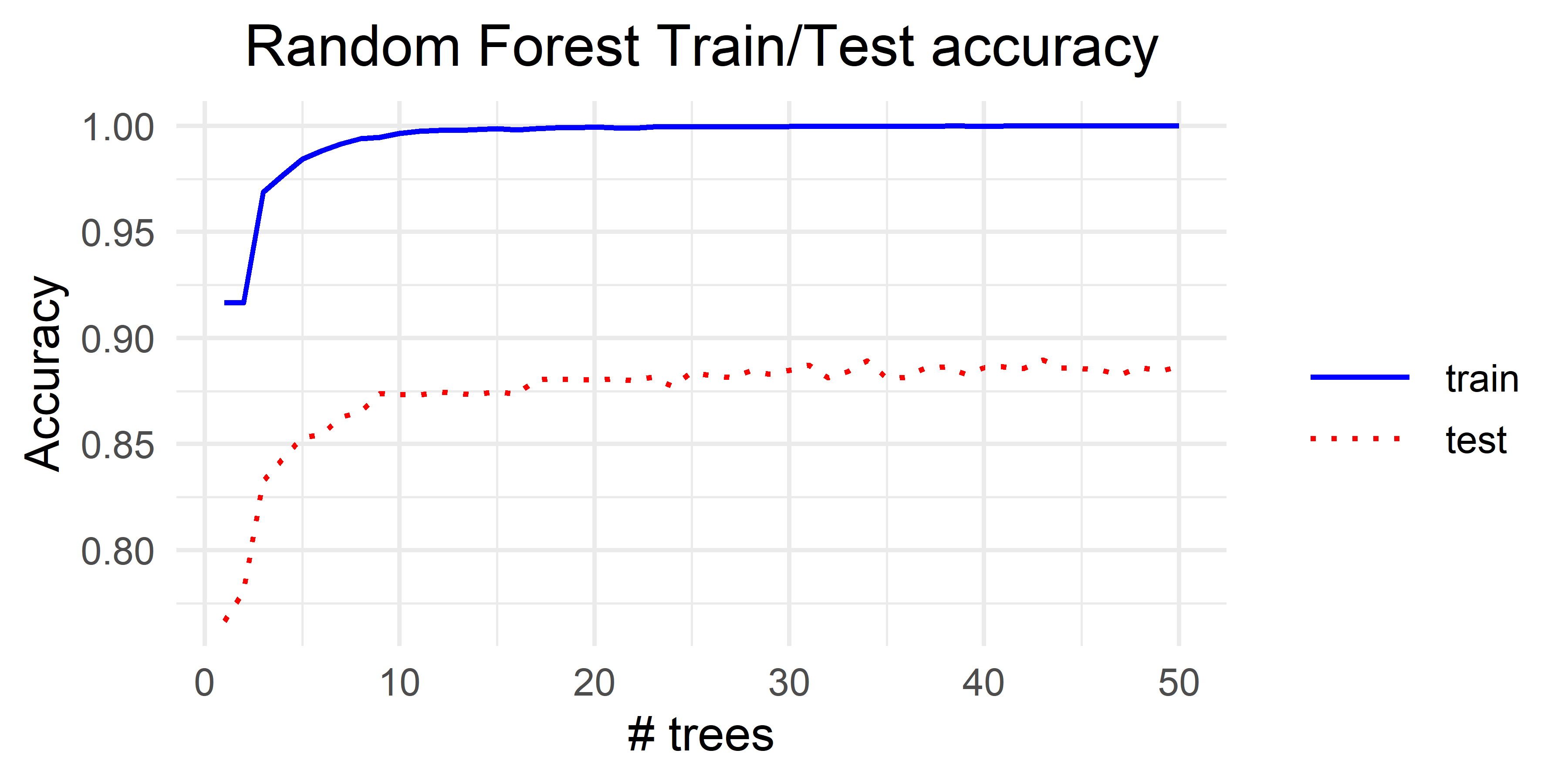
FIGURE 3.3: Random Forest results for different number of trees.
If we directly compare Bagging vs. Random Forest, Random Forest outperforms Bagging (Figure 3.4). The complete code to generate the plot is in the script iterated_bagging_rf.R.
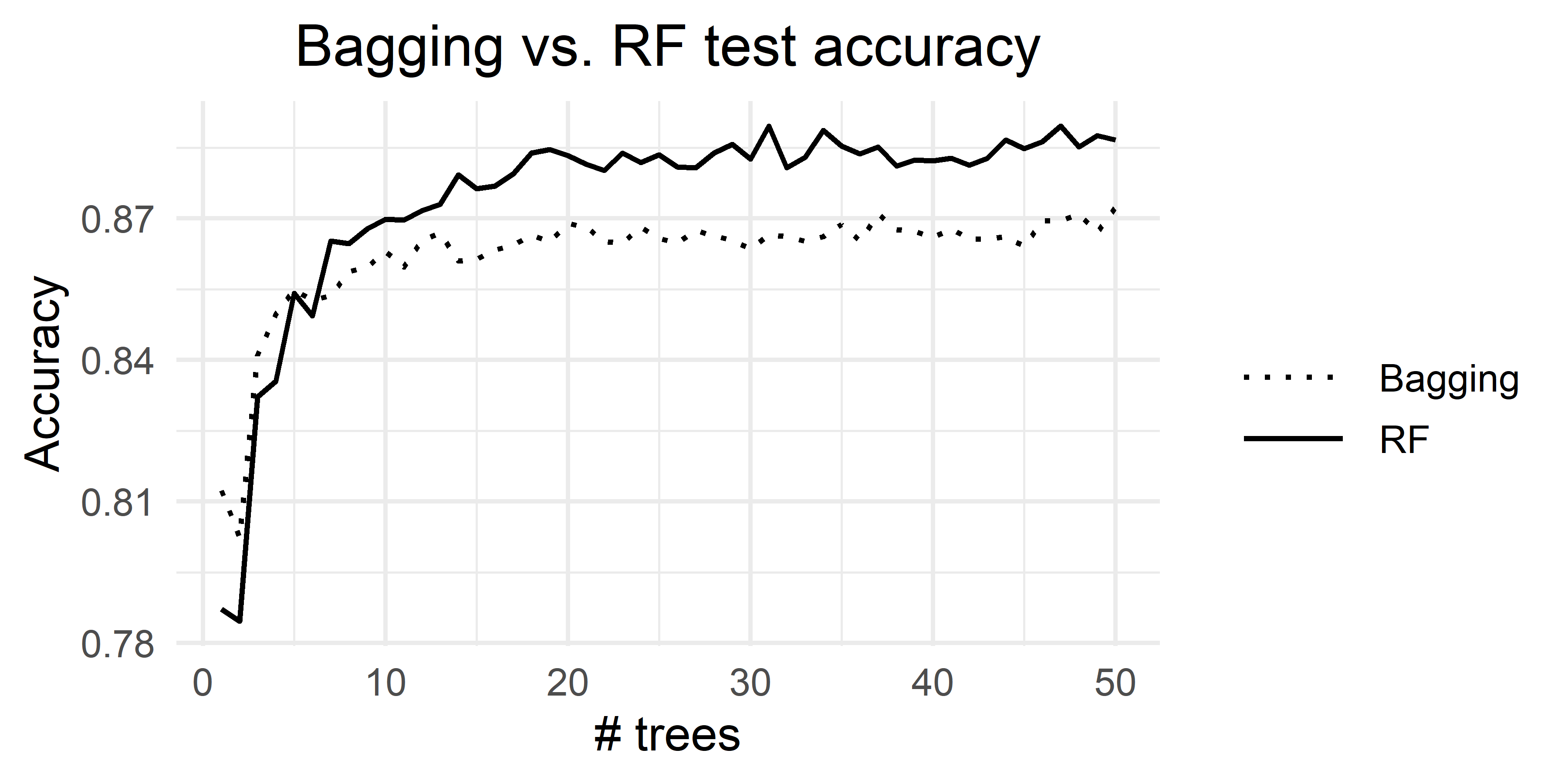
FIGURE 3.4: Bagging vs. Random Forest.
3.3 Stacked Generalization
Stacked Generalization (a.k.a Stacking) is a powerful ensemble learning method proposed by Wolpert (1992). The method consists of training a set of powerful base learners (first-level learners) and combining their outputs by stacking them to form a new train set. The base learners’ outputs are their predictions and optionally, the class probabilities of those predictions. The predictions of the base learners are known as the meta-features. The meta-features along with their true labels \(y\) are used to build a new train set that is used to train a meta-learner. The rationale behind this is that the predictions themselves contain information that can be used by the meta-learner.
The procedure to train a Stacking model is as follows:
Define a set of first level-learners \(\mathscr{L}\) and a meta-learner.
Train the first-level learners \(\mathscr{L}\) with training data \(\textbf{D}\).
Predict the classes of \(\textbf{D}\) with each learner in \(\mathscr{L}\). Each learner produces a predictions vector \(\textbf{p}_i\) with \(\lvert\textbf{D}\lvert\) elements each.
Build a matrix \(\textbf{M}_{\lvert\textbf{D}\lvert \times \lvert\mathscr{L}\lvert}\) by column binding (stacking) the prediction vectors. Then, add the true labels \(\textbf{y}\) to generate the new train set \(\textbf{D}'\).
Train the meta-learner with \(\textbf{D}'\).
Output the final stacking model \(\mathcal{S}:<\mathscr{L},\textit{meta-learner}>\).
Figure 3.5 shows the procedure to generate the new training data \(\textbf{D}'\) used to train the meta-learner.
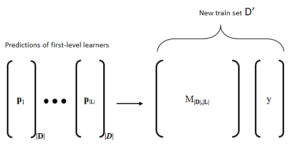
FIGURE 3.5: Process to generate the new train set D’ by column-binding the predictions of the first-level learners and adding the true labels. (Reprinted from Information Fusion Vol. 40, Enrique Garcia-Ceja, Carlos E. Galván-Tejada, and Ramon Brena, “Multi-view stacking for activity recognition with sound and accelerometer data” pp. 45-56, Copyright 2018, with permission from Elsevier, doi: https://doi.org/10.1016/j.inffus.2017.06.004).
Note that steps \(2\) and \(3\) can lead to overfitting because the predictions are made with the same data used to train the models. To avoid this, steps \(2\) and \(3\) are usually performed using \(k\)-fold cross-validation. After \(\textbf{D}'\) has been generated, the learners in \(\mathscr{L}\) can be retrained using all data in \(\textbf{D}\).
Ting and Witten (1999) showed that the performance can increase by adding confidence information about the predictions. For example, the probabilities produced by the first-level learners. Most classifiers can output probabilities.
At prediction time, each first-level learner predicts the class, and optionally, the class probabilities of a given instance. These predictions are used to form a feature vector (meta-features) that is fed to the meta-learner to obtain the final prediction. Usually, first-level learners are high performing classifiers such as Random Forests, Support Vector Machines, Neural Networks, etc. The meta-learner should also be a powerful classifier.
In the next section, I will introduce Multi-view Stacking which is similar to Generalized Stacking except that each first-level learner is trained with features from a different view.
3.4 Multi-view Stacking for Home Tasks Recognition
stacking_algorithms.R stacking_activities.R
Multi-view learning refers to the case when an instance can be characterized by two or more independent ‘views’. For example, one can extract features for webpage classification from a webpage’s text but also from the links pointing to it. Usually, there is the assumption that the views are independent and each is sufficient to solve the problem. Then, why combine them? In many cases, each different view provides additional and complementary information, thus, allowing to train better models.
The simplest thing one can do is to extract features from each view, aggregate them, and train a single model. This approach usually works well but has some limitations. Each view may have different statistical properties, thus, different types of models may be needed for each view. When aggregating features from all views, new variable correlations may be introduced which could impact the performance. Another limitation is that features need to be in the same format (feature vectors, images, etc.), so they can be aggregated.
For video classification, we could have two views. One represented by sequences of images, and the other by the corresponding audio. For the video part, we could encode the features as the images themselves, i.e., matrices. Then, a Convolutional Neural Network (covered in chapter 8) could be trained directly from those images. For the audio part, statistical features can be extracted and stored as normal feature vectors. In this case, the two representations (views) are different. One is a matrix and the other a one-dimensional feature vector. Combining them to train a single classifier could be problematic given the nature of the views and their different encoding formats. Instead, we can train two models, one for each view and then combine the results. This is precisely the idea of Multi-view Stacking (Garcia-Ceja, Galván-Tejada, and Brena 2018). Train a different model for each view and combine the outputs like in Stacking.
Here, Multi-view Stacking will be demonstrated using the HOME TASKS dataset. This dataset was collected from two sources. Acceleration and audio. The acceleration was recorded with a wrist-band watch and the audio using a cellphone. This dataset consists of \(7\) common home tasks: ‘mop floor’, ‘sweep floor’, ‘type on computer keyboard’, ‘brush teeth’, ‘wash hands’, ‘eat chips’, and ‘watch t.v.’. Three volunteers performed each activity for approximately \(3\) minutes.
The acceleration and audio signals were segmented into \(3\)-second windows. From each window, different features were extracted. From the acceleration, \(16\) features were extracted from the \(3\) axes (\(x\),\(y\),\(z\)) such as mean, standard deviation, maximum values, mean magnitude, area under the curve, etc. From the audio signals, \(12\) features were extracted, namely, Mel Frequency Cepstral Coefficients (MFCCs). To preserve volunteers’ privacy, the original audio was not released. The dataset already contains the extracted features from acceleration and audio. The first column is the label.
In order to implement Multi-view Stacking, two Random Forests will be trained, one for each view (acceleration and audio). The predicted outputs will be stacked to form the new training set \(D'\) and a Random Forest trained with \(D'\) will act as the meta-learner.
The next code snippet taken from stacking_algorithms.R shows the multi-view stacking function implemented in R.
mvstacking <- function(D, v1cols, v2cols, k = 10){

  # Generate folds for internal cross-validation.
  folds <- sample(1:k, size = nrow(D), replace = T)

  trueLabels <- NULL
  predicted.v1 <- NULL # predicted labels with view 1
  predicted.v2 <- NULL # predicted labels with view 2
  probs.v1 <- NULL # predicted probabilities with view 1
  probs.v2 <- NULL # predicted probabilities with view 2

  # Perform internal cross-validation.
  for(i in 1:k){

    train <- D[folds != i, ]
    test <- D[folds == i, ]
    trueLabels <- c(trueLabels, as.character(test$label))

    # Train learner with view 1 and make predictions.
    m.v1 <- randomForest(label ~.,
                         train[,c("label",v1cols)], nt = 100)
    raw.v1 <- predict(m.v1, newdata = test[,v1cols], type = "prob")
    probs.v1 <- rbind(probs.v1, raw.v1)
    pred.v1 <- as.character(predict(m.v1,
                                    newdata = test[,v1cols],
                                    type = "class"))
    predicted.v1 <- c(predicted.v1, pred.v1)

    # Train learner with view 2 and make predictions.
    m.v2 <- randomForest(label ~.,
                         train[,c("label",v2cols)], nt = 100)
    raw.v2 <- predict(m.v2, newdata = test[,v2cols], type = "prob")
    probs.v2 <- rbind(probs.v2, raw.v2)
    pred.v2 <- as.character(predict(m.v2,
                                    newdata = test[,v2cols],
                                    type = "class"))
    predicted.v2 <- c(predicted.v2, pred.v2)
  }

  # Build first-order learners with all data.
  learnerV1 <- randomForest(label ~.,
                            D[,c("label",v1cols)], nt = 100)
  learnerV2 <- randomForest(label ~.,
                            D[,c("label",v2cols)], nt = 100)

  # Construct meta-features.
  metaFeatures <- data.frame(label = trueLabels,
                             ((probs.v1 + probs.v2) / 2),
                             pred1 = predicted.v1,
                             pred2 = predicted.v2)

  #train meta-learner
  metalearner <- randomForest(label ~.,
                              metaFeatures, nt = 100)

  res <- structure(list(metalearner=metalearner,
                        learnerV1=learnerV1,
                        learnerV2=learnerV2,
                        v1cols = v1cols,
                        v2cols = v2cols),
                   class = "mvstacking")

  return(res)
}
The first argument D is a data frame containing the training data. v1cols and v2cols are the column names of the two views. Finally, argument k specifies the number of folds for the internal cross-validation to avoid overfitting (Steps \(2\) and \(3\) as described in the generalized stacking procedure).
The function iterates through each fold and trains a Random Forest with the train data for each of the two views. Within each iteration, the trained models are used to predict the labels and probabilities on the internal test set. Predicted labels and probabilities on the internal test sets are concatenated across all folds (predicted.v1, predicted.v2).
After cross-validation, the meta-features are generated by creating a data frame with the predictions of each view. Additionally, the average of class probabilities is added as a meta-feature. The true labels are also added. The purpose of cross-validation is to avoid overfitting but at the end, we do not want to waste data so both learners are re-trained with all data D.
Finally, the meta-learner which is also a Random Forest is trained with the meta-features data frame. A list with all the required information to make predictions is created. This includes first-level learners, the meta-learner, and the column names for each view so we know how to divide the data frame into two views at prediction time.
The following code snippet shows the implementation for making predictions using a trained stacking model.
predict.mvstacking <- function(object, newdata){

  # Predict probabilities with view 1.
  raw.v1 <- predict(object$learnerV1,
                    newdata = newdata[,object$v1cols],
                    type = "prob")

  # Predict classes with view 1.
  pred.v1 <- as.character(predict(object$learnerV1,
                                  newdata = newdata[,object$v1cols],
                                  type = "class"))

  # Predict probabilities with view 2.
  raw.v2 <- predict(object$learnerV2,
                    newdata = newdata[,object$v2cols],
                    type = "prob")

  # Predict classes with view 2.
  pred.v2 <- as.character(predict(object$learnerV2,
                                  newdata = newdata[,object$v2cols],
                                  type = "class"))

  # Build meta-features
  metaFeatures <- data.frame(((raw.v1 + raw.v2) / 2),
                             pred1 = pred.v1,
                             pred2 = pred.v2)

  # Set levels on factors to avoid errors in randomForest predict.
  levels(metaFeatures$pred1) <- object$metalearner$classes
  levels(metaFeatures$pred2) <- object$metalearner$classes

  predictions <- as.character(predict(object$metalearner,
                                      newdata = metaFeatures),
                              type="class")

  return(predictions)
}
The object parameter is the trained model and newdata is a data frame from which we want to make the predictions. First, labels and probabilities are predicted using the two views. Then, a data frame with the meta-features is assembled with the predicted label and the averaged probabilities. Finally, the meta-learner is used to predict the final classes using the meta-features.
The script stacking_activities.R shows how to use our mvstacking() function. With the following two lines we can train and make predictions.
m.stacking <- mvstacking(trainset, v1cols, v2cols, k = 10)
pred.stacking <- predict(m.stacking, newdata = testset[,-1])
The script performs \(10\)-fold cross-validation and for the sake of comparison, it builds three models. One with only audio features, one with only acceleration features, and the Multi-view Stacking one combining both types of features.
Table 3.1 shows the results for each view and with Multi-view Stacking. Clearly, combining both views with Multi-view Stacking achieved the best results compared to using a single view.
| Accuracy | Recall | Specificity | Precision | F1 | |
|---|---|---|---|---|---|
| Audio | 0.8535 | 0.8497 | 0.9753 | 0.8564 | 0.8521 |
| Accelerometer | 0.8557 | 0.8470 | 0.9760 | 0.8523 | 0.8487 |
| Multi-view Stacking | 0.9365 | 0.9318 | 0.9895 | 0.9333 | 0.9325 |
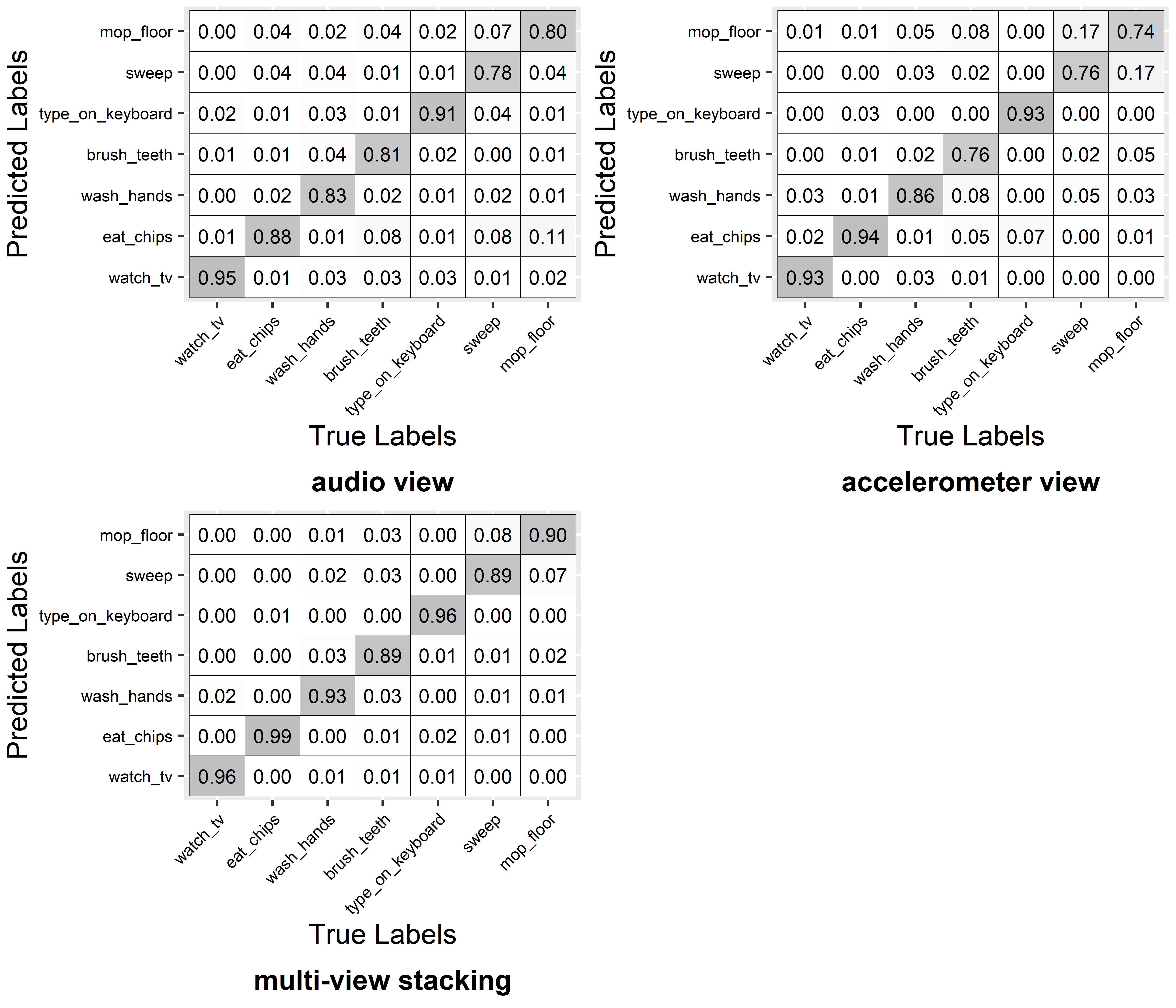
FIGURE 3.6: Confusion matrices.
Figure 3.6 shows the resulting confusion matrices for the three cases. By looking at the recall (anti-diagonal) of the individual classes, it seems that audio features are better at recognizing some activities like ‘sweep’ and ‘mop floor’ whereas the accelerometer features are better for classifying ‘eat chips’, ‘wash hands’, ‘type on keyboard’, etc. thus, those two views are somehow complementary. All recall values when using Multi-view Stacking are higher than for any of the other views.
3.5 Summary
In this chapter, several ensemble learning methods were introduced. In general, ensemble models perform better than single models.
- The main idea of ensemble learning is to train several models and combine their results.
- Bagging is an ensemble method consisting of \(n\) base-learners, each, trained with bootstrapped training samples.
- Random Forest is an ensemble of trees. It introduces randomness to the trees by selecting random features in each split.
- Another ensemble method is called stacked generalization. It consists of a set of base-learners and a meta-learner. The later is trained using the outputs of the base-learners.
- Multi-view learning can be used when an instance can be represented by two or more views (for example, different sensors).