Chapter 1 Introduction to Behavior and Machine Learning

In the last years, machine learning has surged as one of the key technologies that enables and supports many of the services and products that we use in our everyday lives and is expanding quickly. Machine learning has also helped to accelerate research and development in almost every field including natural sciences, engineering, social sciences, medicine, art and culture. Even though all those fields (and their respective sub-fields) are very diverse, most of them have something in common: They involve living organisms (cells, microbes, plants, humans, animals, etc.) and living organisms express behaviors. This book teaches you machine learning and data-driven methods to analyze different types of behaviors. Some of those methods include supervised, unsupervised, and deep learning. You will also learn how to explore, encode, preprocess, and visualize behavioral data. While the examples in this book focus on behavior analysis, the methods and techniques can be applied in any other context.

This chapter starts by introducing the concepts of behavior and machine learning. Next, basic machine learning terminology is presented and you will build your first classification and regression models. Then, you will learn how to evaluate the performance of your models and important concepts such as underfitting, overfitting, bias, and variance.

1.1 What Is Behavior?

Living organisms are constantly sensing and analyzing their surrounding environment. This includes inanimate objects but also other living entities. All of this is with the objective of making decisions and taking actions, either consciously or unconsciously. If we see someone running, we will react differently depending on whether we are at a stadium or in a bank. At the same time, we may also analyze other cues such as the runner’s facial expressions, clothes, items, and the reactions of the other people around us. Based on this aggregated information, we can decide how to react and behave. All this is supported by the organisms’ sensing capabilities and decision-making processes (the brain and/or chemical reactions). Understanding our environment and how others behave is crucial for conducting our everyday life activities and provides support for other tasks. But, what is behavior? The Cambridge dictionary defines behavior as:

“the way that a person, an animal, a substance, etc. behaves in a particular situation or under particular conditions”.

Another definition by dictionary.com is:

“observable activity in a human or animal”.

The definitions are similar and both include humans and animals. Following those definitions, this book will focus on the automatic analysis of human and animal behaviors however, the methods can also be applied to robots and to a wide variety of problems in different domains. There are three main reasons why one may want to analyze behaviors in an automatic manner:

React. A biological or an artificial agent (or a combination of both) can take actions based on what is happening in the surrounding environment. For example, if suspicious behavior is detected in an airport, preventive actions can be triggered by security systems and the corresponding authorities. Without the possibility to automate such a detection system, it would be infeasible to implement it in practice. Just imagine trying to analyze airport traffic by hand.
Understand. Analyzing the behavior of an organism can help us to understand other associated behaviors and processes and to answer research questions. For example, Williams et al. (2020) found that Andean condors, the heaviest soaring bird (see Figure 1.1), only flap their wings for about $1\%$ of their total flight time. In one of the cases, a condor flew $\approx 172$ km without flapping. Those findings were the result of analyzing the birds’ behavior from data recorded by bio-logging devices. In this book, several examples that make use of inertial devices will be studied.

Andean condor. (Hugo Pédel, France, Travail personnel. Cliché réalisé dans le Parc National Argentin Nahuel Huapi, San Carlos de Bariloche, Laguna Tonchek. Source: Wikipedia (CC BY-SA 3.0) [https://creativecommons.org/licenses/by-sa/3.0/legalcode]).

FIGURE 1.1: Andean condor. (Hugo Pédel, France, Travail personnel. Cliché réalisé dans le Parc National Argentin Nahuel Huapi, San Carlos de Bariloche, Laguna Tonchek. Source: Wikipedia (CC BY-SA 3.0) [https://creativecommons.org/licenses/by-sa/3.0/legalcode]).

Document and Archive. Finally, we may want to document certain behaviors for future use. It could be for evidence purposes or maybe it is not clear how the information can be used now but may come in handy later. Based on the archived information, one could gain new knowledge in the future and use it to react (take decisions/actions), as shown in Figure 1.2. For example, we could document our nutritional habits (what do we eat, how often, etc.). If there is a health issue, a specialist could use this historical information to make a more precise diagnosis and propose actions.

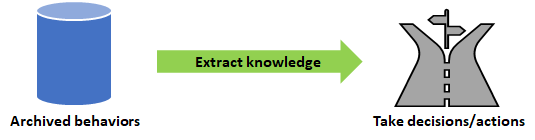
FIGURE 1.2: Taking decisions from archived behaviors.

Some behaviors can be used as a proxy to understand other behaviors, states, and/or processes. For example, detecting body movement behaviors during a job interview could serve as the basis to understand stress levels. Behaviors can also be modeled as a composition of lower-level behaviors. In chapter 7, a method called Bag of Words that can be used to decompose complex behaviors into a set of simpler ones will be presented.

In order to analyze and monitor behaviors, we need a way to observe them. Living organisms use their available senses such as eyesight, hearing, smell, echolocation (bats, dolphins), thermal senses (snakes, mosquitoes), etc. In the case of machines, they need sensors to accomplish or approximate those tasks, for example color and thermal cameras, microphones, temperature sensors, and so on.

The reduction in the size of sensors has allowed the development of more powerful wearable devices. Wearable devices are electronic devices that are worn by a user, usually as accessories or embedded in clothes. Examples of wearable devices are smartphones, smartwatches, fitness bracelets, actigraphy watches, etc. These devices have embedded sensors that allow them to monitor different aspects of a user such as activity levels, blood pressure, temperature, and location, to name a few. Examples of sensors that can be found in those devices are accelerometers, magnetometers, gyroscopes, heart rate, microphones, Wi-Fi, Bluetooth, Galvanic skin response (GSR), etc.

Several of those sensors were initially used for some specific purposes. For example, accelerometers in smartphones were intended to be used for gaming or detecting the device’s orientation. Later, some people started to propose and implement new use cases such as activity recognition (Shoaib et al. 2015) and fall detection. The magnetometer, which measures the earth’s magnetic field, was mainly used with map applications to determine the orientation of the device, but later, it was found that it can also be used for indoor location purposes (Brena et al. 2017).

In general, wearable devices have been successfully applied to track different types of behaviors such as physical activity, sports activities, location, and even mental health states (Garcia-Ceja, Riegler, Nordgreen, et al. 2018). Those devices generate a lot of raw data, but it will be our task to process and analyze it. Doing it by hand becomes impossible given the large amounts of data and their variety. In this book, several machine learning methods will be introduced that will allow you to extract and analyze different types of behaviors from data. The next section will begin with an introduction to machine learning. The rest of this chapter will introduce the required machine learning concepts before we start analyzing behaviors in chapter 2.

1.2 What Is Machine Learning?

You can think of machine learning as a set of computational algorithms that automatically find useful patterns and relationships from data. Here, the keyword is automatic. When trying to solve a problem, one can hard-code a predefined set of rules, for example, chained if-else conditions. For instance, if we want to detect if the object in a picture is an orange or a pear, we can do something like:

if(number_green_pixels > 90%)
  return "pear"
else
  return "orange"

This simple rule should work well and will do the job. Imagine that now your boss tells you that the system needs to recognize green apples as well. Our previous rule will no longer work, and we will need to include additional rules and thresholds. On the other hand, a machine learning algorithm will automatically learn such rules based on the updated data. So, you only need to update your data with examples of green apples and “click” the re-train button!

The result of learning is knowledge that the system can use to solve new instances of a problem. In this case, when you show a new image to the system, it should be able to recognize the type of fruit. Figure 1.3 shows this general idea.

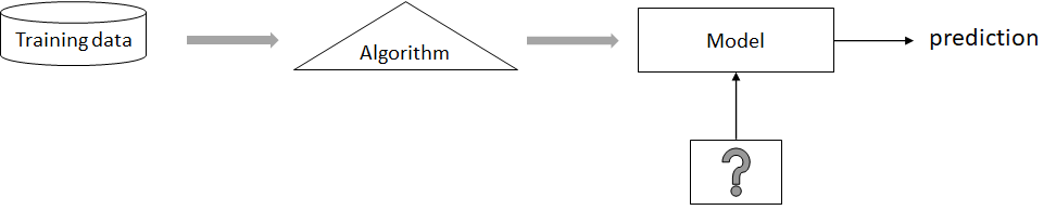
Overall Machine Learning phases. The '?' represents the new unknown object for which we want to obtain a prediction using the learned model.

FIGURE 1.3: Overall Machine Learning phases. The ‘?’ represents the new unknown object for which we want to obtain a prediction using the learned model.

For more formal definitions of machine learning, I recommend you check (Kononenko and Kukar 2007).

Machine learning methods rely on three main building blocks:

Data
Algorithms
Models

Every machine learning method needs data to learn from. For the example of the fruits, we need examples of images for each type of fruit we want to recognize. Additionally, we need their corresponding output types (labels) so the algorithm can learn how to associate each image with its corresponding label.

Not every machine learning method needs the expected output or labels (more on this in the Taxonomy section 1.3).

Typically, an algorithm will use the data to learn a model. This is called the learning or training phase. The learned model can then be used to generate predictions when presented with new data. The data used to train the models is called the train set. Since we need a way to test how the model will perform once it is deployed in a real setting (in production), we also need what is known as the test set. The test set is used to estimate the model’s performance on data it has never seen before (more on this will be presented in section 1.6).

1.3 Types of Machine Learning

Machine learning methods can be grouped into different types. Figure 1.4 depicts a categorization of machine learning ‘types’. This figure is based on (Biecek et al. 2012). The $x$ axis represents the certainty of the labels and the $y$ axis the percent of training data that is labeled. In the previous example, the labels are the names of the fruits associated with each image.

Machine learning taxonomy. (Adapted from Biecek, Przemyslaw, et al. “The R package bgmm: mixture modeling with uncertain knowledge.” Journal of Statistical Software 47.i03 (2012). (CC BY 3.0) [https://creativecommons.org/licenses/by/3.0/legalcode]).

FIGURE 1.4: Machine learning taxonomy. (Adapted from Biecek, Przemyslaw, et al. “The R package bgmm: mixture modeling with uncertain knowledge.” Journal of Statistical Software 47.i03 (2012). (CC BY 3.0) [https://creativecommons.org/licenses/by/3.0/legalcode]).

From the figure, four main types of machine learning methods can be observed:

Supervised learning. In this case, $100\%$ of the training data is labeled and the certainty of those labels is $100\%$. This is like the fruits example. For every image used to train the system, the respective label is also known and there is no uncertainty about the label. When the expected output is a category (the type of fruit), this is called classification. Examples of classification models (a.k.a classifiers) are decision trees, $k$-Nearest Neighbors, Random Forest, neural networks, etc. When the output is a real number (e.g., temperature), it is called regression. Examples of regression models are linear regression, regression trees, neural networks, Random Forest, $k$-Nearest Neighbors, etc. Note that some models can be used for both classification and regression. A supervised learning problem can be formalized as follows:

\[\begin{equation} f\left(x\right) = y \tag{1.1} \end{equation}\]

where $f$ is a function that maps some input data $x$ (for example images) to an output $y$ (types of fruits). Usually, an algorithm will try to learn the best model $f$ given some data consisting of $n$ pairs $(x,y)$ of examples. During learning, the algorithm has access to the expected output/label $y$ for each input $x$. At inference time, that is, when we want to make predictions for new examples, we can use the learned model $f$ and feed it with a new input $x$ to obtain the corresponding predicted value $y$.

Semi-supervised learning. This is the case when the certainty of the labels is $100\%$ but not all training data are labeled. Usually, this scenario considers the case when only a very small proportion of the data is labeled. That is, the dataset contains pairs of examples of the form $(x,y)$ but also examples where $y$ is missing $(x,?)$. In supervised learning, both $x$ and $y$ must be present. On the other hand, semi-supervised algorithms can learn even if some examples are missing the expected output $y$. This is a common situation in real life since labeling data can be expensive and time-consuming. In the fruits example, someone needs to tag every training image manually before training a model. Semi-supervised learning methods try to extract information also from the unlabeled data to improve the models. Examples of some semi-supervised learning methods are self-learning, co-training, and tri-training. (Triguero, García, and Herrera 2013).
Partially-supervised learning. This is a generalization that encompasses supervised and semi-supervised learning. Here, the examples have uncertain (soft) labels. For example, the label of a fruit image instead of being an ‘orange’ or ‘pear’ could be a vector $[0.7, 0.3]$ where the first element is the probability that the image corresponds to an orange and the second element is the probability that it’s a pear. Maybe the image was not very clear, and these are the beliefs of the person tagging the images encoded as probabilities. Examples of models that can be used for partially-supervised learning are mixture models with belief functions (Côme et al. 2009) and neural networks.
Unsupervised learning. This is the extreme case when none of the training examples have a label. That is, the dataset only has pairs $(x,?)$. Now, you may be wondering: If there are no labels, is it possible to extract information from these data? The answer is yes. Imagine you have fruit images with no labels. What you could try to do is to automatically group them into meaningful categories/groups. The categories could be the types of fruits themselves, i.e., trying to form groups in which images within the same category belong to the same type. In the fruits example, we could infer the true types by visually inspecting the images, but in many cases, visual inspection is difficult and the formed groups may not have an easy interpretation, but still, they can be very useful and can be used as a preprocessing step (like in vector quantization). These types of algorithms that find groups (hierarchical groups in some cases) are called clustering methods. Examples of clustering methods are $k$-means, $k$-medoids, and hierarchical clustering. Clustering algorithms are not the only unsupervised learning methods. Association rules, word embeddings, and autoencoders are examples of other unsupervised learning methods. Note: Some people may claim that word embeddings and autoencoders are not fully unsupervised methods but for practical purposes, this is not relevant.

Additionally, there is another type of machine learning called Reinforcement Learning (RL) which has substantial differences from the previous ones. This type of learning does not rely on example data as the previous ones but on stimuli from an agent’s environment. At any given point in time, an agent can perform an action which will lead it to a new state where a reward is collected. The aim is to learn the sequence of actions that maximize the reward. This type of learning is not covered in this book. A good introduction to the topic can be consulted here².

This book will mainly cover supervised learning problems and more specifically, classification problems. For example, given a set of wearable sensor readings, we want to predict contextual information about a given user such as location, current activity, mood, and so on. Unsupervised learning methods (clustering and association rules) will be covered in chapter 6 and autoencoders are introduced in chapter 10.

1.4 Terminology

This section introduces some basic terminology that will be helpful for the rest of the book.

1.4.1 Tables

Since data is the most important ingredient in machine learning, let’s start with some related terms. First, data needs to be stored/structured so it can be easily manipulated and processed. Most of the time, datasets will be stored as tables or in R terminology, data frames. Figure 1.5 shows the classic mtcars dataset³ stored in a data frame.

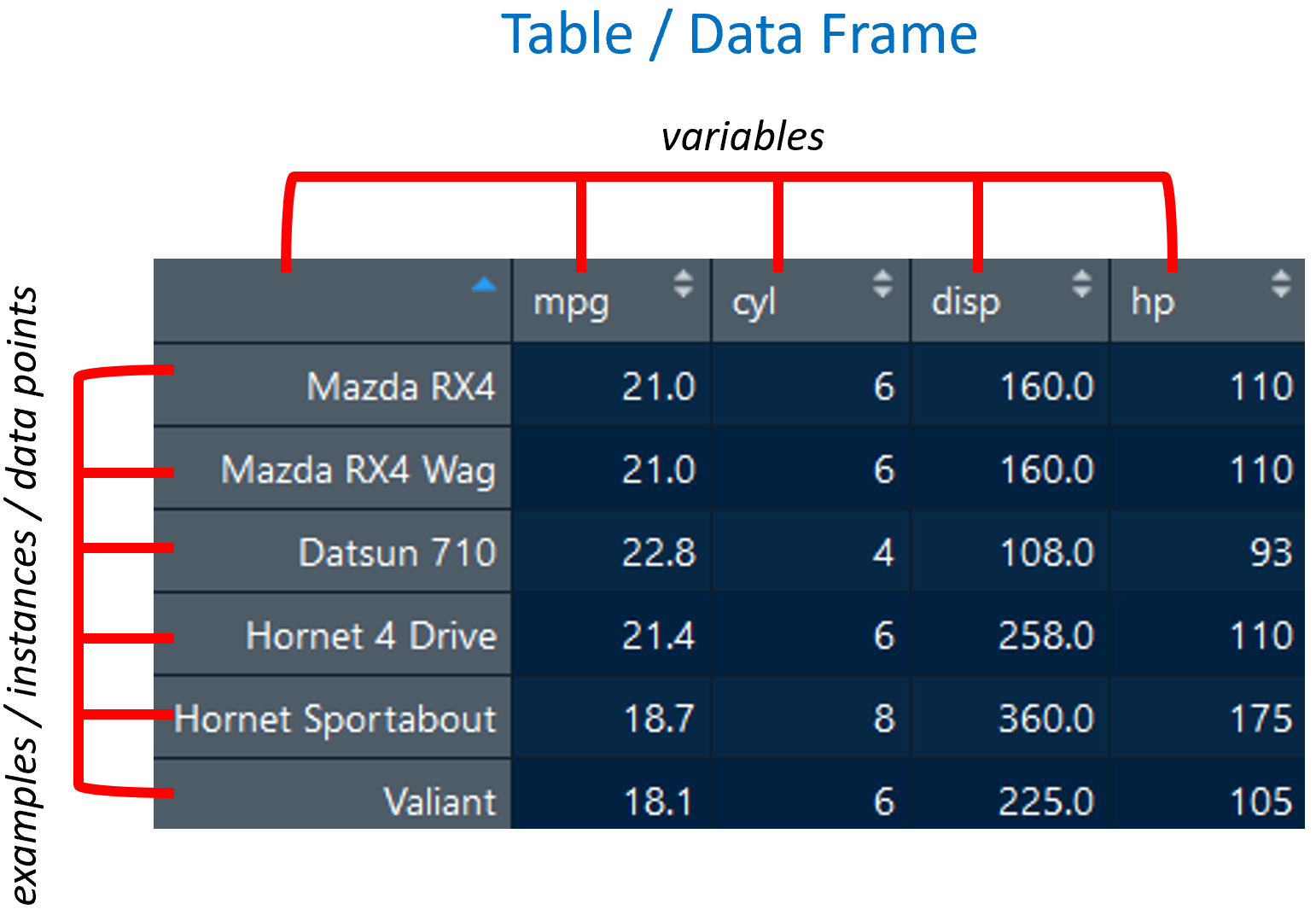
FIGURE 1.5: Table/Data frame components. Source: Data from the 1974 Motor Trend US magazine.

The columns represent variables and the rows represent examples also known as instances or data points. In this table, there are $5$ variables mpg, cyl, disp, hp and the model (the first column). In this example, the first column does not have a name, but it is still a variable. Each row represents a specific car model with its values per variable. In machine learning terminology, rows are more commonly called instances whereas in statistics they are often called data points or observations. Here, those terms will be used interchangeably.

Figure 1.6 shows a data frame for the iris dataset which consists of different kinds of plants (Fisher 1936). Suppose that we are interested in predicting the Species based on the other variables. In machine learning terminology, the variable of interest (the one that depends on the others) is called the class or label for classification problems. For regression, it is often referred to as y. In statistics, it is more commonly known as the response, dependent, or y variable, for both classification and regression.

In machine learning terminology, the rest of the variables are called features or attributes. In statistics, they are called predictors, independent variables, or just X. From the context, most of the time it should be easy to identify dependent from independent variables regardless of the used terminology. The word feature vector is also very common in machine learning. A feature vector is just a structure containing the features of a given instance. For example, the features of the first instance in Figure 1.6 can be stored as a feature vector $[5.4,3.9,1.3,0.4]$ of size $4$. In a programming language, this can be implemented with an array.

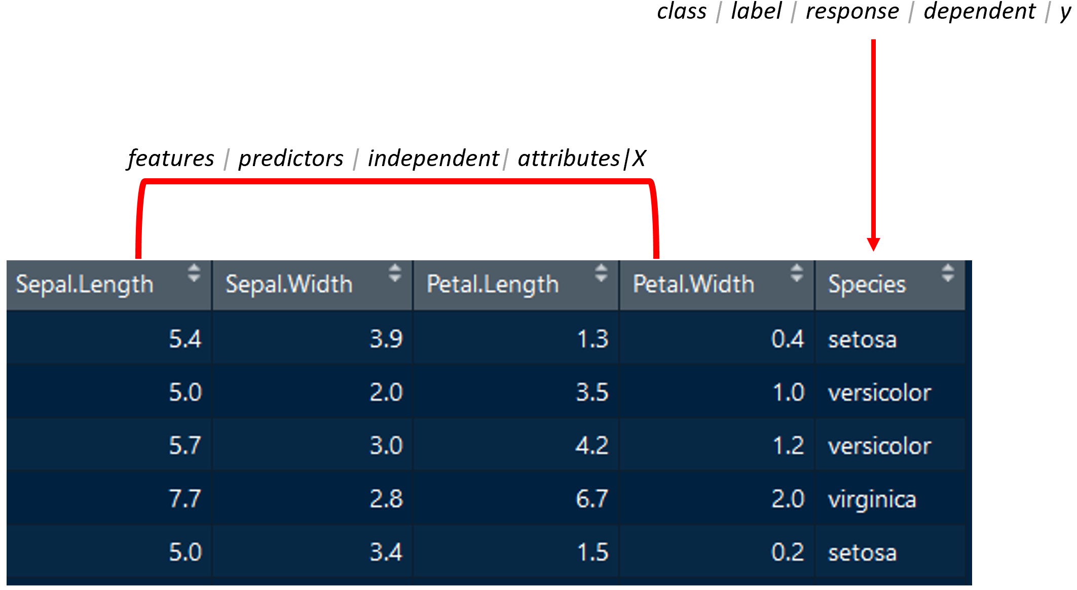
Table/Data frame components (cont.). Source: Data from Fisher, Ronald A., “The Use of Multiple Measurements in Taxonomic Problems.” Annals of Eugenics 7, no. 2 (1936): 179–88.

FIGURE 1.6: Table/Data frame components (cont.). Source: Data from Fisher, Ronald A., “The Use of Multiple Measurements in Taxonomic Problems.” Annals of Eugenics 7, no. 2 (1936): 179–88.

1.4.2 Variable Types

When working with machine learning algorithms, the following are the most commonly used variable types. Here, when I talk about variable types, I do not refer to programming-language-specific data types (int, boolean, string, etc.) but to more general types regardless of the underlying implementation for each specific programming language.

Categorical/Nominal: These variables take values from a discrete set of possible values (categories). For example, the categorical variable color can take the values ‘red’, ‘green’, ‘black’, and so on. Categorical variables do not have an ordering.
Numeric: Real values such as height, weight, price, etc.
Integer: Integer values such as number of rooms, age, number of floors, etc.
Ordinal: Similar to categorical variables, these take their values from a set of discrete values, but they do have an ordering. For example, low < medium < high.

1.4.3 Predictive Models

In machine learning terminology, a predictive model is a model that takes some input and produces an output. Classifiers and Regressors are predictive models. I will use the terms classifier/model and regressor/model interchangeably.

1.5 Data Analysis Pipeline

Usually, the data analysis pipeline consists of several steps which are depicted in Figure 1.7. This is not a complete list but includes the most common steps. It all starts with the data collection. Then the data exploration and so on, until the results are presented. These steps can be followed in sequence, but you can always jump from one step to another one. In fact, most of the time you will end up using an iterative approach by going from one step to the other (forward or backward) as needed.

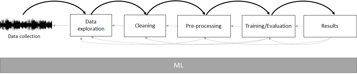
FIGURE 1.7: Data analysis pipeline.

The big gray box at the bottom means that machine learning methods can be used in all those steps and not just during training or evaluation. For example, one may use dimensionality reduction methods in the data exploration phase to plot the data or classification/regression methods in the cleaning phase to impute missing values. Now, let’s give a brief description of each of those phases:

Data exploration. This step aims to familiarize yourself and understand the data so you can make informed decisions during the following steps. Some of the tasks involved in this phase include summarizing your data, generating plots, validating assumptions, and so on. During this phase you can, for example, identify outliers, missing values, or noisy data points that can be cleaned in the next phase. Chapter 4 will introduce some data exploration techniques. Throughout the book, we will also use some other data exploratory methods but if you are interested in diving deeper into this topic, I recommend you check out the “Exploratory Data Analysis with R” book by Peng (2016).
Data cleaning. After the data exploration phase, we can remove the identified outliers, remove noisy data points, remove variables that are not needed for further computation, and so on.
Preprocessing. Predictive models expect the data to be in some structured format and satisfying some constraints. For example, several models are sensitive to class imbalances, i.e., the presence of many instances with a given class but a small number of instances with other classes. In fraud detection scenarios, most of the instances will belong to the normal class but just a small proportion will be of type ‘illegal transaction’. In this case, we may want to do some preprocessing to try to balance the dataset. Some models are also sensitive to feature-scale differences. For example, a variable weight could be in kilograms but another variable height in centimeters. Before training a predictive model, the data needs to be prepared in such a way that the models can get the most out of it. Chapter 5 will present some common preprocessing steps.
Training and evaluation. Once the data is preprocessed, we can proceed to train the models. Furthermore, we also need ways to evaluate their generalization performance on new unseen instances. The purpose of this phase is to try, and fine-tune different models to find the one that performs the best. Later in this chapter, some model evaluation techniques will be introduced.
Interpretation and presentation of results. The purpose of this phase is to analyze and interpret the models’ results. We can use performance metrics derived from the evaluation phase to make informed decisions. We may also want to understand how the models work internally and how the predictions are derived.

1.6 Evaluating Predictive Models

Before showing you how to train a machine learning model, in this section, I would like to introduce the process of evaluating a predictive model, which is part of the data analysis pipeline. This applies to both classification and regression problems. I’m starting with this topic because it will be a recurring one every time you work with machine learning. You will also be training a lot of models, but you will need ways to validate them as well.

Once you have trained a model (with a training set), that is, finding the best function $f$ that maps inputs to their corresponding outputs, you may want to estimate how good the model is at solving a particular problem when presented with examples it has never seen before (that were not part of the training set). This estimate of how good the model is at predicting the output of new examples is called the generalization performance.

To estimate the generalization performance of a model, a dataset is usually divided into a train set and a test set. As the name implies, the train set is used to train the model (learn its parameters) and the test set is used to evaluate/test its generalization performance. We need independent sets because when deploying models in the wild, they will be presented with new instances never seen before. By dividing the dataset into two subsets, we are simulating this scenario where the test set instances were never seen by the model at training time so the performance estimate will be more accurate rather than if we used the same set to train and then to evaluate the performance. There are two main validation methods that differ in the way the dataset is divided into train and test sets: hold-out validation and k-fold cross validation.

1) Hold-out validation. This method randomly splits the dataset into train and test sets based on some predefined percentages. For example, randomly select $70\%$ of the instances and use them as the train set and use the remaining $30\%$ of the examples for the test set. This will vary depending on the application and the amount of data, but typical splits are $50/50$ and $70/30$ percent for the train and test sets, respectively. Figure 1.8 shows an example of a dataset divided into $70/30$.

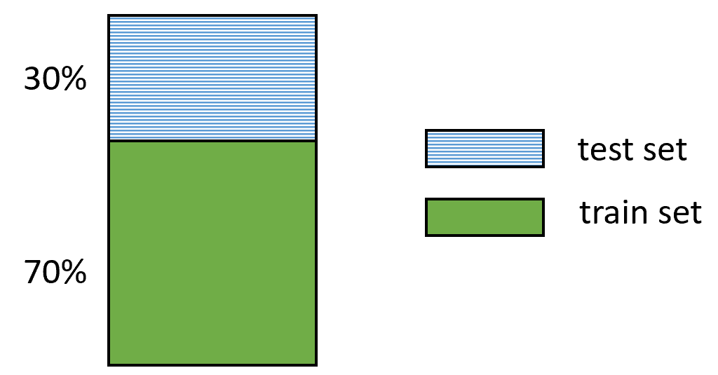
FIGURE 1.8: Hold-out validation.

Then, the train set is used to train (fit) a model, and the test set to evaluate how well that model performs on new data. The performance can be measured using performance metrics such as the accuracy for classification problems. The accuracy is the percent of correctly classified instances.

It is a good practice to estimate the performance on both, the train and test sets. Usually, the performance on the train set will be better since the model was trained with that very same data. It is also common to measure the performance computing the error instead of accuracy. For example, the percent of misclassified instances. These are called the train error and test error (also known as the generalization error), for both the train and test sets, respectively. Estimating these two errors will allow you to ‘debug’ your models and understand if they are underfitting or overfitting (more on this in the following sections).

2) $k$-fold cross-validation. Hold-out validation is a good way to evaluate your models when you have a lot of data. However, in many cases, your data will be limited. In those cases, you want to make efficient use of the data. With hold-out validation, each instance is included either in the train or test set. $k$-fold cross-validation provides a way in which instances take part in both, the test and train set, thus making more efficient use of the data.

This method consists of randomly assigning each instance into one of $k$ folds (subsets) with approximately the same size. Then, $k$ iterations are performed. In each iteration, one of the folds is used to test the model while the remaining ones are used to train it. Each fold is used once as the test set and $k-1$ times as part of the train set. Typical values for $k$ are $3$, $5$, and $10$. In the extreme case where $k$ is equal to the total number of instances in the dataset, it is called leave-one-out cross-validation (LOOCV). Figure 1.8 shows an example of cross-validation with $k=5$.

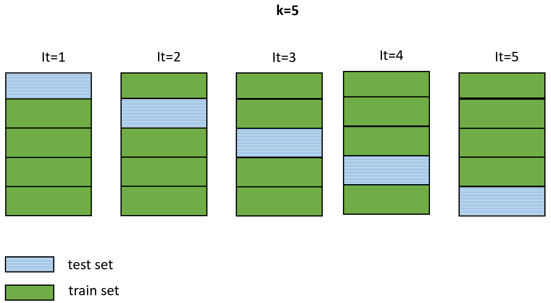
$$k$-fold cross validation with $k=5$ and $5$ iterations.$

FIGURE 1.9: $k$-fold cross validation with $k=5$ and $5$ iterations.

The generalization performance is then computed by taking the average accuracy/error from each iteration.

Hold-out validation is typically used when there is a lot of available data and models take significant time to be trained. On the other hand, $k$-fold cross-validation is used when data is limited. However, it is more computational intensive since it requires training $k$ models.

Validation set.

Most predictive models require some hyperparameter tuning. For example, a $k$-Nearest Neighbors model requires to set $k$, the number of neighbors. For decision trees, one can specify the maximum allowed tree depth, among other hyperparameters. Neural networks require even more hyperparameter tuning to work properly. Also, one may try different preprocessing techniques and features. All those changes affect the final performance. If all those hyperparameter changes are evaluated using the test set, there is a risk of overfitting the model. That is, making the model very specific to this particular data. Instead of using the test set to fine-tune parameters, a validation set needs to be used instead. Thus, the dataset is randomly partitioned into three subsets: train/validation/test sets. The train set is used to train the model. The validation set is used to estimate the model’s performance while trying different hyperparameters and preprocessing methods. Once you are happy with your final model, you use the test set to assess the final generalization performance and this is what you report. The test set is used only once. Remember that we want to assess performance on unseen instances. When using k-fold cross validation, first, an independent test set needs to be put aside. Hyperparameters are tuned using cross-validation and the test set is used at the very end and just once to estimate the final performance.

When working with multi-user systems, we need to additionally take into account between-user differences. In those situations, it is advised to perform extra validations. Those multi-user validation techniques will be covered in chapter 9.

1.7 Simple Classification Example

simple_model.R

So far, a lot of terminology and concepts have been introduced. In this section, we will work through a practical example that will demonstrate how most of these concepts fit together. Here you will build (from scratch) your first classification and regression models! Furthermore, you will learn how to evaluate their generalization performance.

Suppose you have a dataset that contains information about felines including their maximum speed in km/hr and their specific type. For the sake of the example, suppose that these two variables are the only ones that we can observe. As for the types, consider that there are two possibilities: ‘tiger’ and ‘leopard’. Figure 1.10 shows the first $10$ instances (rows) of the dataset.

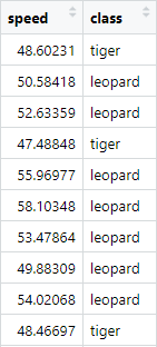
FIGURE 1.10: First 10 instances of felines dataset.

This table has $2$ variables: speed and class. The first one is a numeric variable. The second one is a categorical variable. In this case, it can take two possible values: ‘tiger’ or ‘leopard’.

This dataset was synthetically created for illustration purposes, but I promise you that hereafter, we will mostly use real datasets!

The code to reproduce this example is available in the ‘Introduction to Behavior and Machine Learning’ folder in the script file simple_model.R. The script contains the code used to generate the dataset. The dataset is stored in a data frame named dataset. Let’s start by doing a simple exploratory analysis of the dataset. More detailed exploratory analysis methods will be presented in chapter 4. First, we can print the data frame dimensions with the dim() function.

# Print number of rows and columns.
dim(dataset)
#> [1] 100   2

The output tells us that the data frame has $100$ rows and $2$ columns. Now we may be interested to know how many of those correspond to tigers. We can use the table() function to get that information.

# Count instances in each class.
table(dataset$class)
#> leopard   tiger 
#>      50      50

Here we see that $50$ instances are of type ‘leopard’ and also that $50$ instances are of type ‘tiger’. In fact, this is how the dataset was intentionally generated. The next thing we can do is to compute some summary statistics for each column. R already provides a very convenient function for that purpose. Yes, it is the summary() function.

# Compute some summary statistics.
summary(dataset)
#>      speed           class   
#>  Min.   :42.96   leopard:50  
#>  1st Qu.:48.41   tiger  :50  
#>  Median :51.12               
#>  Mean   :51.53               
#>  3rd Qu.:53.99               
#>  Max.   :61.65

Since speed is a numeric variable, summary() computes some statistics like the mean, min, max, etc. The class variable is a factor. Thus, it returns row counts instead. In R, categorical variables are usually encoded as factors. It is similar to a string, but R treats factors in a special way. We can already appreciate that with the previous code snippet when the summary function returned class counts.

There are many other ways in which you can explore a dataset, but for now, let’s assume we already feel comfortable and that we have a good understanding of the data. Since this dataset is very simple, we won’t need to do any further data cleaning or preprocessing.

Now, imagine that you are asked to build a model that is able to predict the type of feline based on the observed attributes. In this case, the only thing we can observe is the speed. Our task is to build a function that maps speed measurements to classes. That is, we want to be able to predict the type of feline based on how fast it runs. According to the terminology presented in section 1.4, speed would be a feature variable and class would be the class variable.

Based on the types of machine learning methods presented in section 1.3, this one is a supervised learning problem because for each instance, the class is available. And, specifically, since we want to predict a category, this is a classification problem.

Before building our classification model, it would be worth plotting the data. Figure 1.11 shows the speeds for both tigers and leopards.

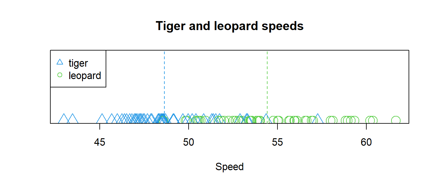
FIGURE 1.11: Feline speeds with vertical dashed lines at the means.

Here, I omitted the code for building the plot, but it is included in the script. I also added vertical dashed lines at the mean speeds for the two classes. From this plot, it seems that leopards are faster than tigers (with some exceptions). One thing we can note is that the data points are grouped around the mean values of their corresponding classes. That is, most of the tiger data points are closer to the mean speed for tigers and the same can be observed for leopards. Of course, there are some exceptions where an instance is closer to the mean of the opposite class. This could be because some tigers may be as fast as leopards. Some leopards may also be slower than the average, maybe because they are newborns or they are old. Unfortunately, we do not have more information, so the best we can do is use our single feature speed. We can use these insights to come up with a simple model that discriminates between the two classes based on this single feature variable.

One thing we can do for any new instance we want to classify is to compute its distance to the ‘center’ of each class and predict the class that is the closest one. In this case, the center is the mean value. We can formally define our model as the set of $n$ centrality measures where $n$ is the number of classes ($2$ in our example).

\[\begin{equation} M = \{\mu_1,\dots ,\mu_n\} \tag{1.2} \end{equation}\]

Those centrality measures (the class means in this particular case) are called the parameters of the model. Training a model consists of finding those optimal parameters that will allow us to achieve the best performance on new instances that were not part of the training data. In most cases, we will need an algorithm to find those parameters. In our example, the algorithm consists of simply computing the mean speed for each class. That is, for each class, sum all the corresponding speeds and divide them by the number of data points that belong to that class.

Once those parameters are found, we can start making predictions on new data points. This is called inference or prediction. In this case, when a new data point arrives, we can predict its class by computing its distance to each of the $n$ centrality measures in $M$ and return the class of the closest one.

The following function implements the training part of our model.

# Define a simple classifier that learns
# a centrality measure for each class.
simple.model.train <- function(data, centrality=mean){
  
  # Store unique classes.
  classes <- unique(data$class)
  
  # Define an array to store the learned parameters.
  params <- numeric(length(classes))
  
  # Make this a named array.
  names(params) <- classes
  
  # Iterate through each class and compute its centrality measure.
  for(c in classes){
    
    # Filter instances by class.
    tmp <- data[which(data$class == c),]
    
    # Compute the centrality measure.
    centrality.measure <- centrality(tmp$speed)
    
    # Store the centrality measure for this class.
    params[c] <- centrality.measure
  }
  
  return(params)
}

The first argument is the training data and the second argument is the centrality function we want to use (the mean, by default). This function iterates each class, computes the centrality measure based on the speed, and stores the results in a named array called params which is then returned at the end.

Most of the time, training a model involves feeding it with the training data and any additional hyperparameters specific to each model. In this case, the centrality measure is a hyperparameter and here, we set it to be the mean.

The difference between parameters and hyperparameters is that the former are learned during training. The hyperparameters are settings specific to each model that can be defined before the actual training starts.

Now that we have a function that performs the training, we need another one that performs the actual inference or prediction on new data points. Let’s call this one simple.classifier.predict(). Its first argument is a data frame with the instances we want to get predictions for. The second argument is the named vector of parameters learned during training. This function will return an array with the predicted class for each instance in newdata.

# Define a function that predicts a class
# based on the learned parameters.
simple.classifier.predict <- function(newdata, params){
  
  # Variable to store the predictions of
  # each instance in newdata.
  predictions <- NULL
  
  # Iterate instances in newdata
  for(i in 1:nrow(newdata)){
    
    instance <- newdata[i,]
    
    # Predict the name of the class which
    # centrality measure is closest.
    pred <- names(which.min(abs(instance$speed - params)))
    
    predictions <- c(predictions, pred)
  }
  
  return(predictions)
}

This function iterates through each row and computes the distance to each centrality measure and returns the name of the class that was the closest one. The distance computation is done with the following line of code:

pred <- names(which.min(abs(instance$speed - params)))

First, it computes the absolute difference between the speed and each centrality measure stored in params and then, it returns the class name of the minimum one. Now that we have defined the training and prediction procedures, we are ready to test our classifier!

In section 1.6, two evaluation methods were presented. Hold-out and k-fold cross-validation. These methods allow you to estimate how your model will perform on new data. Let’s start with hold-out validation.

First, we need to split the data into two independent sets. We will use $70\%$ of the data to train our classifier and the remaining $30\%$ to test it. The following code splits dataset into a trainset and testset.

# Percent to be used as training data.
pctTrain <- 0.7

# Set seed for reproducibility.
set.seed(123)

idxs <- sample(nrow(dataset),
               size = nrow(dataset) * pctTrain,
               replace = FALSE)

trainset <- dataset[idxs,]

testset <- dataset[-idxs,]

The sample() function was used to select integer numbers at random from $1$ to $n$, where $n$ is the total number of data points in dataset. These randomly selected data points are the ones that will go to the train set. The size argument tells the function to return $70$ numbers which correspond to $70\%$ of the total since dataset has $100$ instances.

The last argument replace is set to FALSE because we do not want repeated instances. The ‘-’ symbol in dataset[-idxs,] is used to select everything that is not in the train set. This ensures that any instance only belongs to either the train or the test set. We don’t want an instance to be copied into both sets.

Now it’s time to test our functions. We can train our model using the trainset by calling our previously defined function simple.model.train().

# Train the model using the trainset.
params <- simple.model.train(trainset, mean)

# Print the learned parameters.
print(params)
#>    tiger  leopard 
#> 48.88246 54.58369

After training the model, we print the learned parameters. In this case, the mean for tiger is $48.88$ and for leopard, it is $54.58$. With these parameters, we can start making predictions on our test set! We pass the test set and the newly-learned parameters to our function simple.classifier.predict().

# Predict classes on the test set.
test.predictions <- simple.classifier.predict(testset, params)

# Display first predictions.
head(test.predictions)
#> [1] "tiger"   "tiger"   "leopard" "tiger"   "tiger"   "leopard"

Our predict function returns predictions for each instance in the test set. We can use the head() function to print the first predictions. The first two instances were classified as tigers, the third one as leopard, and so on.

But how good are those predictions? Since we know what the true classes are (also known as ground truth) in our test set, we can compute the performance. In this case, we will compute the accuracy, which is the percentage of correct classifications. Note that we did not use the class information when making predictions, we only used the speed. We pretended that we didn’t have the true class. We will use the true class only to evaluate the model’s performance.

# Compute test accuracy.
sum(test.predictions == as.character(testset$class)) /
  nrow(testset)
#> [1] 0.8333333

We can compute the accuracy by counting how many predictions were equal to the true classes and divide them by the total number of points in the test set. In this case, the test accuracy was $83.0\%$. Congratulations! you have trained and evaluated your first classifier.

It is also a good idea to compute the performance on the same train set that was used to train the model.

# Compute train accuracy.
train.predictions <- simple.classifier.predict(trainset, params)
sum(train.predictions == as.character(trainset$class)) /
  nrow(trainset)
#> [1] 0.8571429

The train accuracy was $85.7\%$. As expected, this was higher than the test accuracy. Typically, what you report is the performance on the test set, but we can use the performance on the train set to look for signs of over/under-fitting which will be covered in the following sections.

1.7.1 $k$-fold Cross-validation Example

Now, let’s see how $k$-fold cross-validation can be implemented to test our classifier. I will choose a $k=5$. This means that $5$ independent sets are going to be generated and $5$ iterations will be run.

# Number of folds.
k <- 5

set.seed(123)

# Generate random folds.
folds <- sample(k, size = nrow(dataset), replace = TRUE)

# Print how many instances ended up in each fold.
table(folds)
#> folds
#>  1  2  3  4  5 
#> 21 20 23 17 19

Again, we can use the sample() function. This time we want to select random integers between $1$ and $k$. The total number of integers will be equal to the total number of instances $n$ in the entire dataset. Note that this time we set replace = TRUE since $k < n$, so this implies that we need to pick repeated numbers. Each number will represent the fold to which each instance belongs to. As before, we need to make sure that each instance belongs only to one of the sets. Here, we are guaranteeing that by assigning each instance a single fold number. We can use the table() function to print how many instances ended up in each fold. Here, we see that the folds will contain between $17$ and $23$ instances.

$k$-fold cross-validation consists of iterating $k$ times. In each iteration, one of the folds is selected as the test set and the remaining folds are used to build the train set. Within each iteration, the model is trained with the train set and evaluated with the test set. At the end, the average accuracy across folds is reported.

# Variables to store accuracies on each fold.
test.accuracies <- NULL
train.accuracies <- NULL

for(i in 1:k){
  testset <- dataset[which(folds == i),]
  trainset <- dataset[which(folds != i),]
  
  params <- simple.model.train(trainset, mean)
  test.predictions <- simple.classifier.predict(testset, params)
  train.predictions <- simple.classifier.predict(trainset, params)
  
  # Accuracy on test set.
  acc <- sum(test.predictions == 
               as.character(testset$class)) /
    nrow(testset)
  
  test.accuracies <- c(test.accuracies, acc)
  
  # Accuracy on train set.
  acc <- sum(train.predictions == 
               as.character(trainset$class)) /
    nrow(trainset)
  
  train.accuracies <- c(train.accuracies, acc)
}

# Print mean accuracy across folds on the test set.
mean(test.accuracies)
#> [1] 0.829823

# Print mean accuracy across folds on the train set.
mean(train.accuracies)
#> [1] 0.8422414

The test mean accuracy across the $5$ folds was $\approx 83\%$ which is very similar to the accuracy estimated by hold-out validation.

Note that in section 1.6 a validation set was also mentioned. This one is useful when you want to fine-tune a model and/or try different preprocessing methods on your data. In case you are using hold-out validation, you may want to split your data into three sets: train/validation/test sets. So, you train your model using the train set and estimate its performance using the validation set. Then you can fine-tune your model. For example, here, instead of the mean as centrality measure, you can try to use the median and measure the performance again with the validation set. When you are pleased with your settings, you estimate the final performance of the model with the test set only once.

In the case of $k$-fold cross-validation, you can set aside a test set at the beginning. Then you use the remaining data to perform cross-validation and fine-tune your model. Within each iteration, you test the performance with the validation data. Once you are sure you are not going to do any parameter tuning, you can train a model with the train and validation sets and test the generalization performance using the test set.

One of the benefits of machine learning is that it allows us to find patterns based on data freeing us from having to program hard-coded rules. This means more scalable and flexible code. If for some reason, now, instead of $2$ classes we needed to add another class, for example, a ‘jaguar’, the only thing we need to do is update our database and retrain our model. We don’t need to modify the internals of the algorithms. They will update themselves based on the data.

We can try this by adding a third class ‘jaguar’ to the dataset as shown in the script simple_model.R. It then trains the model as usual and performs predictions.

1.8 Simple Regression Example

simple_model.R

As opposed to classification models where the aim is to predict a category, regression models predict numeric values. To exemplify this, we can use our felines dataset but instead try to predict speed based on the type of feline. The class column will be treated as a feature variable and speed will be the response variable. Since there is only one predictor, and it is categorical, the best thing we can do to implement our regression model is to predict the mean speed depending on the class.

Recall that for the classification scenario, our learned parameters consisted of the means for each class. Thus, we can reuse our training function simple.model.train(). All we need to do is to define a new predict function that returns the speed based on the class. This is the opposite of what we did in the classification case (return the class based on the speed).

# Define a function that predicts speed
# based on the type of feline.
simple.regression.predict <- function(newdata, params){
  
  # Variable to store the predictions of
  # each instance in newdata.
  predictions <- NULL
  
  # Iterate instances in newdata
  for(i in 1:nrow(newdata)){
    
    instance <- newdata[i,]
    
    # Return the mean value of the corresponding class stored in params.
    pred <- params[which(names(params) == instance$class)]
    
    predictions <- c(predictions, pred)
  }
  
  return(predictions)
}

The simple.regression.predict() function iterates through each instance in newdata and returns the mean speed from params for the corresponding class.

Again, we can validate our model using hold-out validation. The train set will contain $70\%$ of the instances and the remaining will be used as the test set.

pctTrain <- 0.7
set.seed(123)
idxs <- sample(nrow(dataset),
               size = nrow(dataset) * pctTrain,
               replace = FALSE)

trainset <- dataset[idxs,]
testset <- dataset[-idxs,]

# Reuse our train function.
params <- simple.model.train(trainset, mean)

print(params)
#>    tiger  leopard 
#> 48.88246 54.5836

Here, we reused our previous function simple.model.train() to learn the parameters and then print them. Then we can use those parameters to infer the speed. If a test instance belongs to the class ‘tiger’ then return $48.88$. If it is of class ‘leopard’ then return $54.58$.

# Predict speeds on the test set.
test.predictions <- 
  simple.regression.predict(testset, params)

# Print first predictions.
head(test.predictions)
#> 48.88246 54.58369 54.58369 48.88246 48.88246 54.58369

Since these are numeric predictions, we cannot use accuracy as in the classification case to evaluate the performance. One way to evaluate the performance of regression models is by computing the mean absolute error (MAE). This measure tells you, on average, how much each prediction deviates from its true value. It is computed by subtracting each prediction from its real value and taking the absolute value: $|predicted - realValue|$. This can be visualized in Figure 1.12. The distances between the true and predicted values are the errors and the MAE is the average of all those errors.

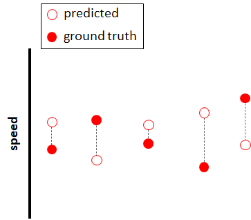
FIGURE 1.12: Prediction errors.

We can use the following code to compute the MAE:

# Compute mean absolute error (MAE) on the test set.
mean(abs(test.predictions - testset$speed))
#> [1] 2.562598

The MAE on the test set was $2.56$. That is, on average, our simple model had a deviation of $2.56$ km/hr with respect to the true values, which is not bad. We can also compute the MAE on the train set.

# Predict speeds on the train set.
train.predictions <- 
  simple.regression.predict(trainset, params)

# Compute mean absolute error (MAE) on the train set.
mean(abs(train.predictions - trainset$speed))
#> [1] 2.16097

The MAE on the train set was $2.16$, which is better than the test set MAE (small MAE values are preferred). Now, you have built, trained, and evaluated a regression model!

This was a simple example, but it illustrates the basic idea of regression and how it differs from classification. It also shows how the performance of regression models is typically evaluated with the MAE as opposed to the accuracy used in classification. In chapter 8, more advanced methods such as neural networks will be introduced, which can be used to solve regression problems.

In this section, we have gone through several of the data analysis pipeline phases. We did a simple exploratory analysis of the data and then we built, trained, and validated the models to perform both classification and regression. Finally, we estimated the overall performance of the models and presented the results. Here, we coded our models from scratch, but in practice, you typically use models that have already been implemented and tested. All in all, I hope these examples have given you the feeling of how it is to work with machine learning.

1.9 Underfitting and Overfitting

From the felines classification example, we saw how we can separate two classes by computing the mean for each class. For the two-class problem, this is equivalent to having a decision line between the two means (Figure 1.13). Everything to the right of this decision line will be closer to the mean that corresponds to ‘leopard’ and everything to the left to ‘tiger’. In this case, the classification function is a vertical line. During learning, the position of the line that reduces the classification error is searched for. We implicitly estimated the position of the line by finding the mean values for each of the classes.

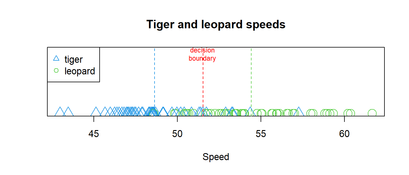
FIGURE 1.13: Decision line between the two classes.

Now, imagine that we do not only have access to the speed but also to the felines’ age. This extra information could help us reduce the prediction error since age plays an important role in how fast a feline is. Figure 1.14 (left) shows how it will look like if we plot age in the x-axis and speed in the y-axis. Here, we can see that for both, tigers and leopards, the speed seems to increase as age increases. Then, at some point, as age increases the speed begins to decrease.

Constructing a classifier with a single vertical line as we did before will not work in this $2$-dimensional case where we have $2$ predictors. Now we will need a more complex decision boundary (function) to separate the two classes. One approach would be to use a line as before but this time we allow the line to have a slope (angle). Everything below the line is classified as ‘tiger’ and everything else as ‘leopard’. Thus, the learning phase involves finding the line’s position and its slope that achieves the smallest error.

Figure 1.14 (left) shows a possible decision line. Even though this function is more complex than a vertical line, it will still produce a lot of misclassifications (it does not clearly separate both classes). This is called underfitting, that is, the model is so simple that it is not able to capture the underlying data patterns.

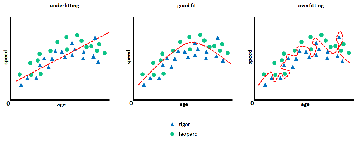
FIGURE 1.14: Underfitting and overfitting.

Let’s try a more complex function, for example, a curve. Figure 1.14 (middle) shows that a curve does a better job at separating the two classes with fewer misclassifications but still, $3$ leopards are misclassified as tigers and $1$ tiger is misclassified as leopard. Can we do better than that? Yes, just keep increasing the complexity of the decision function.

Figure 1.14 (right) shows a more complex function that was able to separate the two classes with $100\%$ accuracy or equivalently, with a $0\%$ error. However, there is a problem. This function learned how to accurately separate the training data, but it is likely that it will not do as well with a new test set. This function became so specialized with respect to this particular data that it failed to capture the overall pattern. This is called overfitting. In this case, the model ‘memorizes’ the train set instead of finding general patterns applicable to new unseen instances. If we were to choose a model, the best one would be the one in the middle. Even if it is not perfect on the train data, it will do better than the other models when evaluated on new test data.

Overfitting is a common problem in machine learning. One way to know if a model is overfitting is by checking if the error in the train set is low while it is high on a new set (can be a test or validation set). Figure 1.15 illustrates this idea. Too-simple models will produce a high error for both, the train and validation sets (underfitting). As the complexity of the model increases, the errors on both sets are reduced. Then, at some point, the complexity of a model becomes so high that it gets too specific on the train set and fails to perform well on a new independent set (overfitting).

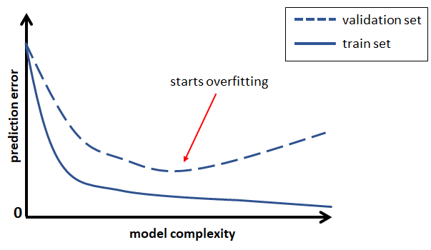
FIGURE 1.15: Model complexity vs. train and validation error.

In this example, we saw how underfitting and overfitting can affect the generalization performance of a model in a classification setting but the same can occur in regression problems.

There are several methods that aim to reduce overfitting, but many of them are specific to the type of model. For example, with decision trees (covered in chapter 2), one way to reduce overfitting is to limit their depth or build ensembles of trees (chapter 3). Neural networks are also highly prone to overfitting since they can be very complex and have millions of parameters. In chapter 8, several techniques to reduce the effect of overfitting will be presented.

1.10 Bias and Variance

So far, we have seen how to train predictive models and evaluate how well they do on new data (test/validation sets). The main goal is to have predictive models that have a low error rate when used with new data. Understanding the source of the error can help us make more informed decisions when building predictive models. The test error, also known as the generalization error of a predictive model can be decomposed into three components: bias, variance, and noise.

Noise. This component is inherent to the data itself and there is nothing we can do about it. For example, two instances having the same values in their features but with a different label.

Bias. How much the average prediction differs from the true value. Note the average keyword. This means that we make the assumption that an infinite (or very large) number of train sets can be generated and for each, a predictive model is trained. Then we average the predictions of all those models and see how much that average differs from the true value.

Variance. How much the predictions change for a given data point when training a model using a different train set each time.

Bias and variance are closely related to underfitting and overfitting. High variance is a sign of overfitting. That is, a model is so complex that it will fit a particular train set very well. Every time it is trained with a different train set, the train error will be low, but it will likely generate very different predictions for the same test points and a much higher test error.

Figure 1.16 illustrates the relation between overfitting and high variance with a regression problem.

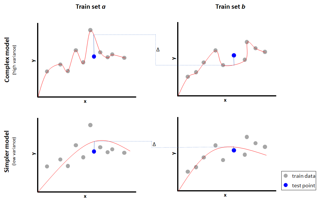
FIGURE 1.16: High variance and overfitting.

Given a feature $x$, two models are trained to predict $y$: i) a complex model (top row), and ii) a simpler model (bottom row). Both models are fitted with two training sets ($a$ and $b$) sampled from the same distribution. The complex model fits the train data perfectly but makes very different predictions (big $\Delta$) for the same test point when using a different train set. The simpler model does not fit the train data so well but has a smaller $\Delta$ and a lower error on the test point as well. Visually, the function (red curve) of the complex model also varies a lot across train sets whereas the shapes of the simpler model functions look very similar.

On the other hand, if a model is too simple, it will underfit causing highly biased results without being able to capture the input-output relationships. This results in a high train error and in consequence, a high test error as well.

A formal definition of the error decomposition is explained in the book “The elements of statistical learning: data mining, inference, and prediction” (Hastie, Tibshirani, and Friedman 2009).

1.11 Summary

In this chapter, several introductory machine learning concepts and terms were introduced and they are the basis for the methods that will be covered in the following chapters.

Behavior can be defined as “an observable activity in a human or animal”.
Three main reasons of why we may want to analyze behavior automatically were discussed: react, understand, and document/archive.
One way to observe behavior automatically is through the use of sensors and/or data.
Machine Learning consists of a set of computational algorithms that automatically find useful patterns and relationships from data.
The three main building blocks of machine learning are: data, algorithms, and models.
The main types of machine learning are supervised learning, semi-supervised learning, partially-supervised learning, and unsupervised learning.
In R, data is usually stored in data frames. Data frames have variables (columns) and instances (rows). Depending on the task, variables can be independent or dependent.
A predictive model is a model that takes some input and produces an output. Classifiers and regressors are predictive models.
A data analysis pipeline consists of several tasks including data collection, cleaning, preprocessing, training/evaluation, and presentation of results.
Model evaluation can be performed with hold-out validation or $k$-fold cross-validation.
Overfitting occurs when a model ‘memorizes’ the training data instead of finding useful underlying patterns.
The test error can be decomposed into noise, bias, and variance.

References

Biecek, Przemyslaw, Ewa Szczurek, Martin Vingron, Jerzy Tiuryn, et al. 2012. “The r Package Bgmm: Mixture Modeling with Uncertain Knowledge.” Journal of Statistical Software 47 (i03).

Brena, Ramon F, Juan Pablo Garcı́a-Vázquez, Carlos E Galván-Tejada, David Muñoz-Rodriguez, Cesar Vargas-Rosales, and James Fangmeyer. 2017. “Evolution of Indoor Positioning Technologies: A Survey.” Journal of Sensors 2017: 1–22.

Côme, Etienne, Latifa Oukhellou, Thierry Denoeux, and Patrice Aknin. 2009. “Learning from Partially Supervised Data Using Mixture Models and Belief Functions.” Pattern Recognition 42 (3): 334–48.

Fisher, Ronald A. 1936. “The Use of Multiple Measurements in Taxonomic Problems.” Annals of Eugenics 7 (2): 179–88.

Garcia-Ceja, Enrique, Michael Riegler, Tine Nordgreen, Petter Jakobsen, Ketil J Oedegaard, and Jim Tørresen. 2018. “Mental Health Monitoring with Multimodal Sensing and Machine Learning: A Survey.” Pervasive and Mobile Computing.

Hastie, Trevor, Robert Tibshirani, and Jerome Friedman. 2009. The Elements of Statistical Learning: Data Mining, Inference, and Prediction. New York, New York: Springer Science & Business Media.

Kononenko, Igor, and Matjaz Kukar. 2007. Machine Learning and Data Mining. Horwood Publishing.

Peng, Roger. 2016. Exploratory Data Analysis with r. Leanpub.com.

Shoaib, Muhammad, Stephan Bosch, Ozlem Durmaz Incel, Hans Scholten, and Paul J. M. Havinga. 2015. “A Survey of Online Activity Recognition Using Mobile Phones.” Sensors 15 (1): 2059–85. https://doi.org/10.3390/s150102059.

Triguero, Isaac, Salvador García, and Francisco Herrera. 2013. “Self-Labeled Techniques for Semi-Supervised Learning: Taxonomy, Software and Empirical Study.” Knowledge and Information Systems 42 (2): 245–84. https://doi.org/10.1007/s10115-013-0706-y.

Williams, HJ, ELC Shepard, Mark D Holton, PAE Alarcón, RP Wilson, and SA Lambertucci. 2020. “Physical Limits of Flight Performance in the Heaviest Soaring Bird.” Proceedings of the National Academy of Sciences.

http://www.scholarpedia.org/article/Reinforcement_learning ↩︎
mtcars dataset https://stat.ethz.ch/R-manual/R-patched/library/datasets/html/mtcars.html extracted from the 1974 Motor Trend US magazine.↩︎

Behavior Analysis with Machine Learning Using R